[Table of Contents]
[Next Article]
Forecasts of Surface Air Temperature and Precipitation
Using GISS SI95 Model Driven by SST and Soil Moisture Anomalies
contributed by GISS Summer Institute Pinatubo Group
NASA Goddard Institute for Space Studies, New
York, New York
GISS climate modeling focuses on decadal time scales.
But testing of our model on seasonal predictions has potential research
and educational benefits. Just as simulations of paleoclimate are invaluable
for checking our model and our understanding, seasonal forecasting provides
an equally useful, different, test which may help us develop an improved
model.
The GISS Institute on Climate and Planets involves New
York City students and educators in GISS research projects. The Pinatubo
project is studying the causes of climate variations in the period 1979şpresent,
including the roles of unforced or chaotic variability and climate forcings.
The GISS SI95 Climate Model
The Pinatubo group "froze" a version (SI95)
of the GISS atmospheric GCM in 1995 and made a series of model runs for
the period 1979ş1995 in which four measured radiative forcings (stratospheric
aerosols, ozone, other greenhouse gases, and solar irradiance) were added
oneşbyşone. The runs using all of these forcings were repeated with four
different ways of treating the ocean: (A) observed SSTs, (B) Qşflux ocean,
(C) "GISS" dynamical ocean (Russell et al. 1995), and (D) "GFDL"
dynamical ocean (Bryan and Cox 1972). For each case an ensemble of five
runs was carried out. The model and experiments are described in a paper
being written during the 1996 GISS Summer Institute (Hansen et al. 1996b),
which will be submitted to the Journal of Geophysical Research.
The SI95 version of the GISS atmospheric GCM is improved
considerably over GISS model II (Hansen et al. 1983). In addition to higher
spatial resolution (4 x 5 degrees) and higher accuracy numerical methods
[quadratic upstream scheme, equivalent to that of Prather (1986), for heat
and moisture and fourth order differencing for the momentum and mass equations
(Abram-opoulos 1991)], the greatest changes are in the PBL (Hartke and
Rind 1996), clouds (Del Genio et al. 1996), moist convection (Del Genio
and Yao 1993) and ground hydrology (Rosenzweig and Abramopoulos 1996).
The model including all the major changes has been documented in several
papers and AMIP intercomparisons, as delineated by Hansen et al. (1996b).
Perhaps the most relevant intercomparison for U. S. forecasts is that of
Boyle (1996), which shows that the current GISS model is among the more
realistic models.
Predictability and Expected Forecast Skill
The simulations for 1979ş1995 with observed timeşvarying SSTs, with and without the four observed radiative forcings, were compared with observations and with simulations using climatological SSTs, as discussed in our paper in preparation (Hansen et al. 1996b). The results suggest that the interannual variability of seasonal mean temperature and precipitation on this 17 year time scale is principally unforced (chaotic) variability. However there is a significant dependence on the boundary forcings, and thus potential predictability, which is much higher at low latitudes than high latitudes, higher for temperature than precipitation, higher in the summer than in the winter, and higher in some years than in others. For example, SSTs seemed to have had a relatively large influence on climate in the United States during the summer of 1988, when the SSTs were characterized by unusual, large, anomalies, while the SSTs of the early 1990s seemed to provide less predictability. In addition, sensitivity tests with arbitrary changes to springtime soil moisture indicated substantial impact on simulated climate of the following summer.
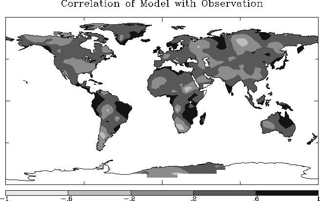
A measure of the model's skill is provided by global maps
of the correlation of the simulation ensembleşmean with observations for
the period 1979ş1995. Such a map is shown by Hansen et al. (1996b) for
tropospheric temperature, based on MSU (Microwave Sounding Unit) channel
2 observations. The correlation for the Jun-Jul-Aug seasonal mean exceeds
0.7 in much of the tropics and varies from about 0.3 at the U.S.şCanada
border to 0.6 at the southern border of the U.S. Correlations with surface
air temperature are lower (Fig. 1), about 0.2 over the U.S. and 0.6 in
the tropics. The very low value over the U.S. is partly a fluke of this
particular 5şrun ensemble, as 5şrun ensembles with other radiative forcings
yield correlations of 0.3ş0.4 there. Correlation skill for precipitation
(not shown) is lower on an overall global basis than that for temperature.
This measure of predictability is optimistic, because
it is based on use of simultaneous observed monthly SSTs, while the forecast
must predict or extrapolate SSTs for three months. On the other hand, it
may be possible to exceed this level of predictability by making use of
added information such as initial conditions of soil moisture. Soil moisture
should be a particularly relevant variable in summer, and its random variability
in the 17şyear runs may be a principal reason for the low predictability
of surface temperature.
Seasonal forecast experiments;
Forecasts for Jun-Jul-Aug 1996
No tuning of the model was made for the seasonal forecasts,
as the original calibrations were carried out with respect to the decadal
time scale. We simply extended for three months the model simulations that
used observed SSTs. The results that we show are anomalies calculated relative
to the model's 12şyear base period 1979ş1990. We show results for two 5şmember
ensembles. Ensemble A specifies SST as climatology plus the anomalies observed
in the last week of May 1996, with no attempt to predict changes of SST
anomalies during Jun-Jul-Aug. Ensemble B adds an estimate of soil moisture
anomalies on June 1, as described below. Both ensembles include radiative
forcings as extrapolations of recent observations, but these have very
little impact on seasonal climate variability (Hansen 1996a,b).
Ensemble A yields a precipitation deficit and high temperatures
in the U.S. Southwest in June (Fig. 2). Qualitatively similar results were
obtained in May and June in an ensemble of runs initiated May 1 (not illustrated).
We have not determined the formal significance of the calculated climate
anomalies for the summer of 1996. The June temperature anomaly in the Southwestşsouthcentral
U.S. may be significant, as it has the same sign in four of the five runs
and was comparably strong in the ensemble initiated May 1. But in July
and August of these ensembles there is a similar frequency of above normal
and below normal precipitation and temperature, at face value suggesting
that there is a good chance of the drought breaking during the summer.
Among the first qualifications of such a prediction is
the question of whether the model includes a realistic soil moisture anomaly
at the beginning of the summer, given the sensitivity of seasonal simulations
to initial soil moisture inferred by other investigators (e.g., Betts et
al. 1996) and also found in sensitivity studies with our model. Thus we
carried out a second ensemble of experiments (Ensemble B, Fig. 3) in which
we specified a soil moisture anomaly for June 1 based on an approximate
Palmer Drought Index (PDI). PDI was calculated from monthly means of precipitation
and temperature in preceding months, based on a program provided by Tom
Karl and Richard Knight of NCDC. The scale factor required to convert a
PDI anomaly to a soil moisture anomaly was set by requiring that the mean
magnitude of the soil moisture anomalies equal the mean magnitude of soil
moisture anomalies in the model's climatology. In regions without monthly
mean data (principally the Amazon basin and the Sahara) the soil moisture
anomaly on June 1 is that which was generated by the 17 year model run.
Ensemble B yields a much different forecast in the U.S.,
with a stronger heat and drought anomaly persisting through June, July
and August. This testifies again to the sensitivity of regional climate
to soil moisture anomalies in our model. In the 5şrun means there are obvious
geographical correlations of simulated climate anomalies with soil moisture
initial conditions. This positive feedback is at variance with conclusions
of Giorgi et al. (1996) based on a mesoscale model, but consistent with
the analysis of Betts et al. (1996) and with previous sensitivity studies
with our model (Hansen et al. 1996b) and other models.
Interpretation and Discussion
We emphasize that our model has not been designed for
regional forecasting. These "forecasts" are not intended for
operational purposes, but rather have objectives related to research and
education. Our aim is to help understand the significance of different
mechanisms in regional climate fluctuations and to improve the realism
of our climate model.
The simulations suggest that SST anomalies, possibly the
proximate large warm region off the west coast of the U.S., may have been
an immediate cause of the current drought in the southwest and south-central
U.S. It will be of interest to examine the meteorology associated with
the anomalies, quantify their significance, and perhaps do experiments
to geographically isolate the effective forcing.
The simulations with only SST forcing would suggest
that there is a good chance of the drought in the southwest U.S. breaking
in JulyşAugust. But inclusion of an initial soil moisture anomaly inferred
from a drought index tilts the prediction toward continuation of the drought.
Indeed, these simulations suggest that the drought area will expand during
the course of the summer.
Although the sense of the soil moisture impact on the
forecast seems reasonable, its magnitude suggests that both the procedure
for obtaining the soil moisture anomaly and the ground hydrology scheme
in the GISS GCM should be carefully scrutinized. The 6şlayer hydrology
scheme (Rosenzweig and Abramopoulos 1996) includes shallow, intermediate,
and deep layers which encompass a range of time constants and a large moisture
field capacity.
Perhaps the main issue raised by these forecast experiments
concerns the role and time constant of soil moisture anomalies. Either
our estimation of the initial anomalies is excessive, or our model unrealistically
magnifies the impact of soil moisture, or soil moisture has a greater impact
on climate forecasts than is generally believed. If the soil moisture impact
is indeed large, is it also possible that the deep soil layers have an
effect on interannual time scales?
Both forecast experiments produce some strong anomalies
at low latitudes, including below normal temperatures and heavy precipitation
in Northeast Brazil and the Sahel. The model has high skill in Northeast
Brazil in the period 1979ş95 (correlation 0.6ş0.7 for temperature, 0.5ş0.6
for precipitation), but low skill in the Sahel (about 0.2 for temperature,
0.0 for precipita-tion). The excess precipitation in Northeast Brazil and
the low temperatures in both places are consistent with expectations for
a La Nina period (Ropelewski and Halpert 1987; Halpert and Ropelewski 1992),
although climate anomalies in these regions are also dependent on SST anomalies
in the Atlantic (Ward and Folland 1991, Hastenrath and Greischar 1993,
Lamb and Peppler 1991).
The present simulations are intended only to study the
impact of SSTs and soil moisture on predictability. We do not attempt to
initialize atmospheric conditions in our model: the June 1 atmospheric
conditions were not used; the model picked up the atmospheric conditions
already in progress from the 1979 start time. We also do not use a very
high resolution, as would be required for optimal shortşterm forecasting.
Even the two boundary conditions that we examine are handled crudely. One
potential improvement would be to replace the fixed SST anomalies with
predicted SSTs. This is probably essential for forecasts of more than a
few months, and may be an important factor even in single season forecasts.
Our simulations also point out the need to determine soil moisture initial
conditions more accurately. Although observations of global soil moisture
do not appear to be practical at present, it should be possible to use
the time history of precipitation and temperature to generate improved
soil moisture initial conditions as a function of depth. Empirical use
of such calculated soil moisture for long-range temperature prediction
has been discussed in this Bulletin (June 1995) and in Huang et al. (1996).
Acknowledgments: The paper in preparation (Hansen
et al. 1996b), describing the SI95 model and experiments, will include
a large number of collaborators at other NASA centers and universities.
Tom Karl and Dick Knight of NOAA NCDC kindly provided a program for calculating
a drought index from monthly precipitation and temperature.
References
Abramopoulos, F., 1991: A new fourthşorder enstrophy and
energy conserving scheme, Mon. Wea. Rev., 119, 128ş133.
Betts, A.K., J.H. Hall, A.C.M. Beljaars, M.J. Miller and P.A. Viterbo, 1996: The landşsurface- atmosphere interaction, J. Geophys. Res., 101, 7209ş7225.
Boyle, J.S., 1996: Seasonal characteristics of precipitation
over the United States in AMIP simulations. PCMDI Report No. 31, Lawrence
Livermore Laboratory, Livermore, California, 30 pp.
Bryan, K. and M.D. Cox, 1972: An approximate equation
of state for numerical model of ocean circulation, J. Phys. Oceanogr.,
15, 1255ş1273.
Del Genio, A.D. and M.S. Yao, 1993: Efficient cumulus
parameterization for longşterm climate studies: GISS scheme, AMS Mono.,
46, 181ş184.
Del Genio, A.D., M.S. Yao, W. Kovari, and K.K. Lo, 1996:
A prognostic cloud water parameterization for global climate models, J.
Climate, 9, in press.
Giorgi, F., L. Mearns, C. Shields and L. Mayer, 1996:
A regional model study of the importance of local versus remote controls
of the 1988 drought and the 1993 flood over the central United States,
J. Climate., 9, 1150ş1162.
Halpert, M.S. and C.F. Ropelewski, 1992: Surface temperature
patterns associated with the Southern Oscillation, J. Climate, 5,
577-593.
Hansen, J., G. Russell, D. Rind, P. Stone, A. Lacis, S.
Lebedeff, R. Ruedy, and L. Travis, 1983: Efficient threeşdimensional global
models for climate studies: models I and II, Mon. Wea. Rev., 111,
609ş662.
Hansen, J., M. Sato, R. Ruedy, A. Lacis, K. Asamoah, S.
Borenstein, E. Brown, B. Cairns, G. Caliri, M. Campbell, B. Curran, S.
de Castro, L. Druyan, M. Fox, C. Johnson, J. Lerner, M.P. McCormick, R.
Miller, P. Minnis, A. Morrison, L. Pandolfo, I. Ramberran, F. Zaucker,
M. Robinson, P. Russell, K. Shah, P. Stone, I. Tegen, L. Thomason, J. Wilder,
and H. Wilson, 1996a: A Pinatubo climate modeling investigation, in NATO
ASI Series Volume, Subseries I Global Environment Change,
Eds. G. Fiocco, D. Fua and G. Viscount, SpringerşVerlag.
Hansen, J. and APinatubo Team@, 1996b: Forcings and chaos
in interannual to decadal climate change, J. Geophys Res, to be
submitted.
Hartke, G.J. and D. Rind: An improved boundary layer model
for the GISS GCM, 1996: J. Climate, 9, in press.
Hastenrath, S. and L. Greischar, 1993: Further work on
the prediction of northeast Brazil rainfall anomalies. J. Climate,
6, 743-758.
Huang, J., H.M. van den Dool and K.P. Georgakakos, 1996:
Analysis of model-calculated soil moisture over the United States (1931-1993)
and applications to long-range temperature forecasts. J. Climate,
9, in press (to be in July or August issue).
Lamb, P. and R. Peppler, 1991: West Africa. Chapter 5.
In Teleconnections: Linkages between ENSO, Worldwide Climate Anomalies,
and Societal Impacts. M.H. Glantz. R.W. Katz, N. Nicholls, Eds., Cambridge
University Press, 121-189.
Prather, M.J., 1986: Numerical advection by conservation
of second order moments. J. Geophys. Res., 91, 6671ş6680.
Ropelewski, C.F. and M.S. Halpert, 1987: Global and regional
scale precipitation patterns associated with ENSO, Mon. Wea. Rev.,
115, 1606ş1626.
Rosenzweig, C. and F. Abramopoulos, 1996: Land surface
model development for the GISS GCM, J. Climate, in press.
Russell, G.L., J. Miller and D. Rind, 1995: A coupled
atmosphereşocean model for transient climate change studies, Atmos.
Ocean, 33, 687ş730.
Ward, M.N., and C.K. Folland, 1991: Prediction of seasonal
rainfall in the North Nordeste of Brazil using eigenvectors of sea surface
temperature. Int. J. Climatol., 11, 711-743.
Fig. 1. Correlation of observed 1979ş1995 Jun-Jul-Aug
surface air temperature (MSU channel 2) with 5şrun mean of model simulations,
the model being forced by simultaneous observed SSTs.
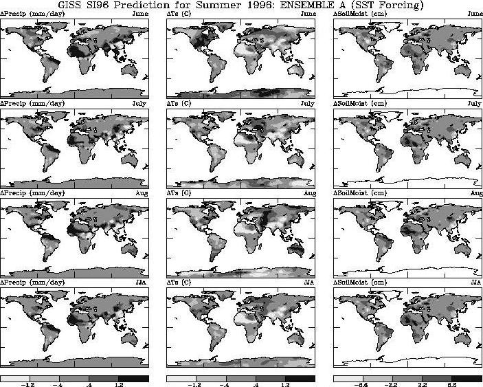
Fig. 2. Temperature (left), precipitation (center),
and soil moisture mean anomalies for Ensemble A (SST forcing) simulations
of summer months (Jun-Jul-Aug) of 1996.
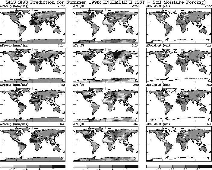
Fig. 3. Same as Fig. 1, but for Ensemble B simulations
(SST forcing + soil moisture anomaly).
________________
*Subset of "Pinatubo" group preparing summer forecast, prior to arrival of most high school participants:
J. Hansen, K. Beckford, S. Borenstein, E. Brown, B. Cairns, S. DeCastro,
L. Druyan, M. Kelly, A. Luckett, R. Miller, R. Ruedy, and J. Wilder.