[Next Article] -
[Previous Article]
Consolidated Forecasts of Tropical Pacific SST
in Niño 3.4 Using Two Dynamical Models and Two Statistical
Models
contributed by David Unger, Anthony Barnston, Huug van den Dool and Vern Kousky
Climate Prediction Center, NOAA, Camp Springs, Maryland
In this Bulletin we find a fairly large number of
forecasts for the east-central tropical Pacific SST for
the coming year. Some predict continuation of the
current cold episode throughout 1996. Others forecast
a rapid dissipation, followed by varying degrees of
warming as boreal winter 1996-97 approaches. The
direction of the forecast is not related to the type of
model--either statistical or dynamical models may go
either way. Which models are we to believe this time,
or any time?
One approach to the problem is to combine, or
consolidate, the forecasts of several models into a single
forecast. This could be done on the basis of the past
behavior of each contributing model, as well as the
overlap of information among the models. There are
several methods by which this can be done. A common
method, and the one used here, is linear multiple
regression. In effect, a statistical scheme is used to
combine outputs of entire models whose natures
themselves may be statistical, dynamical, or a mixture
of the two. In this case we use four input models. Two
are dynamical: the Lamont-Doherty Earth
Observatory's simple coupled model (the improved
LDEO2; Chen et al. 1995; Cane and Zebiak 1986), and
the NCEP coupled model (Ji et al. 1994). The other two
models are statistical: the NCEP constructed analogue
(CA) model (Van den Dool 1994; Van den Dool and
Barnston 1995), and the NCEP canonical correlation
analysis (CCA) model (Barnston 1994). The individual
forecasts of each model are shown elsewhere in this
Bulletin issue.
To derive the multiple regression equations for
each target season for each lead time, histories of the
forecasts of each model were obtained. The CCA and
CA models have histories covering 1956-1995. The
Lamont coupled model has a 1972-95 history, and the
NCEP coupled model 1982-95. To circumvent the
problem of the differing units and climatologies used,
all forecasts were converted to actual C forecasts. The
observations were expressed likewise. The regressions
are based on forecasts for the Niño 3.4 region (5N-5S, 120-170W), except for the Lamont model, from
which we receive forecasts for the Niño 3 region. The
Niño 3 forecast histories from the Lamont model were
used as a predictor for Niño 3.4 in the equation
development. The regression coefficients compensate
for the slight differences between Niño 3 and Niño 3.4
to obtain the least squares fit for Niño 3.4. We expect
to begin receiving gridded forecast fields from Lamont
shortly, and will then be able to use Lamont's Niño 3.4
forecasts directly.
The desired lead times of the consolidated
forecasts range from 0.5 months to 12.5 months by 1
month increments, where lead time is defined as the
time skipped between the time of the forecast and the
beginning of the forecasted (target) period. For
example, the forecasts shown here, which are issued in
the middle of March 1996, have target periods
including Apr-May-Jun 1996, May-Jun-Jul 1996, ...,
Apr-May-Jun 1997. Three of the four individual models
have forecast histories whose leads range to 12.5
months or greater, while one (the NCEP coupled
model) has a maximum lead of only 7.5 months.
Consolidated forecasts for lead times higher than 7.5
months, therefore, are based only on the other three
models; a slight discontinuity in the forecast time series
may thus be expected between the Nov-Dec-Jan and the
Dec-Jan-Feb 1996-97 forecasts.
Because the NCEP coupled model forecast only
has a 1982-95 history, the training period for the
regression is limited to that period and thus results in
greater uncertainty in the coefficients than would be the
case if a longer history could be used. When that model
is not included in the consolidation process for the
longer lead times, the 1972-95 period is used to derive
the regression equations, making for a more favorable
training sample.
The consolidated forecast for Niño 3.4 resulting
from the multiple regression run in mid-March 1996,
expressed as a standardized anomaly, is shown in Fig. 1.
The box and whisker intervals for the forecasts at each
time indicate the one and two error standard deviation,
based on estimated skill following shrinkage of the
dependent sample skill results in accordance with the
sample size and number of predictors. The SST is
expected to remain cold through fall 1996 before
returning to normal in early spring 1997 and then
switching to a weak positive anomaly.
Examination of the regression coefficients reveals
that the statistical models are relatively heavily weighted
in boreal winter. The Lamont model is the most heavily
weighted input for target periods in and around boreal
summer. The CCA and CA models, whose forecasts are
fairly highly positively correlated (>0.8 during the cold
season when their skills are highest), often create some
instability in the coefficients such that one of them
(usually CA) is positively weighted while the other
(CCA) is negatively weighted by roughly the same
magnitude. This instability could be alleviated by (1)
eliminating one of the two statistical models, (2) forming
a simple combination (e.g. an average) of the CCA and
CA forecasts prior to the regression, or (3) keeping both
models but "ridging" the diagonal of the variance-covariance matrix (increasing the diagonal elements) to
make for a more stable matrix inversion. Presently we do
not entirely understand the problem or its solution, and
are studying these. We do know that the amount of
colinearity between CA and CCA is not enormous.
In the present forecast, intuition is lacking in the
sense that as CCA predicts rising SST between spring
and fall of 1996, its negative regression weight
contributes to the decrease in the consolidated forecast in
that time interval (Fig. 1). In the coming months the
consolidation procedure will be further developed and, it
is hoped, made more trustworthy as well as intuitively
reasonable.
Acknowledgments: We are grateful to Stephen
Zebiak and Mark Cane of Lamont Doherty Earth
Observatory, and Ming Ji and Ants Leetmaa from the
National Centers for Environmental Prediction, for
providing the forecast histories from their respective
dynamical models, as well as their current real-time
forecasts.
References
Barnston, A.G., 1994: Linear statistical short-term
climate predictive skill in the Northern Hemisphere. J.
Climate, 5, 1514-1564.
Cane, M., S.E. Zebiak and S.C. Dolan, 1986:
Experimental forecasts of El Nino. Nature, 321,
827-832.
Chen, D., S.E. Zebiak, A.J. Busalacchi and M.A.
Cane, 1995:An improved procedure for El Nino
forecasting: Implications for predictability. Science, 269,
1699-1702.
Ji, M., A. Kumar and A. Leetmaa, 1994: An
experimental coupled forecast system at the National
Meteorological Center: Some early results. Tellus, 46A,
398-418.
van den Dool, H.M., 1994: Searching for
analogues, how long must we wait? Tellus, 46A,
314-324.
van den Dool, H.M. and A.G. Barnston, 1995:
Forecasts of global sea surface temperature out to a year
using the constructed analogue method. Proceedings of
the 19th Annual Climate Diagnostics Workshop,
November 14-18, 1994, College Park, Maryland, 416-419.
Figures
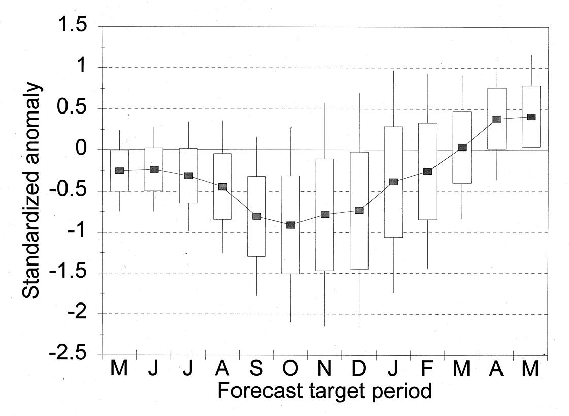 Figure 1. Consolidated forecast
for the standardized anomaly of the SST in the Ni¤o 3.4 region
(5řN-5řS, 120-170řW) for the next 13 running 3-month period. Month
labels on the abscissa denote the middle month of the 3-month
predictand periods. Box and whiskers for each point forecast indicate
the one and two error standard deviation intervals, based on estimated
cross-validated skill.
Figure 1. Consolidated forecast
for the standardized anomaly of the SST in the Ni¤o 3.4 region
(5řN-5řS, 120-170řW) for the next 13 running 3-month period. Month
labels on the abscissa denote the middle month of the 3-month
predictand periods. Box and whiskers for each point forecast indicate
the one and two error standard deviation intervals, based on estimated
cross-validated skill.
[Purpose] -
[Contents] -
[Editorial Policy] -
[Next Article] -
[Previous Article]