Based on this intercomparison as discussed in the EMC assessment, plus the results presented below, we summarize the PAOBS problem as follows:
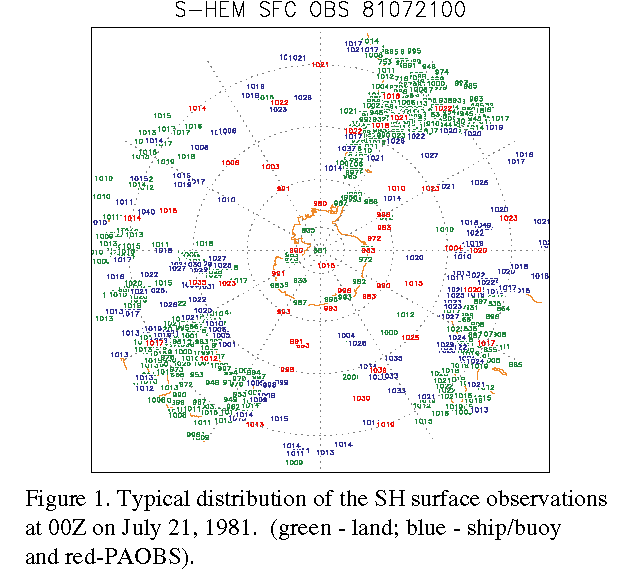
Below we explore the impact of the PAOBS mislocation on the SH middle and high latitudes during July 1981; results from July 1979 are presented in the EMC posting. For reference, a typical distribution of the SH surface observations during July 1981 is shown in Fig. 1 (green - land; blue - ship/buoy and red-PAOBS). Also, we note that when the PAOBS are used correctly, roughly 90% pass the quality control of the assimilation system; when the PAOBS are mislocated, roughly 50% are assimilated.
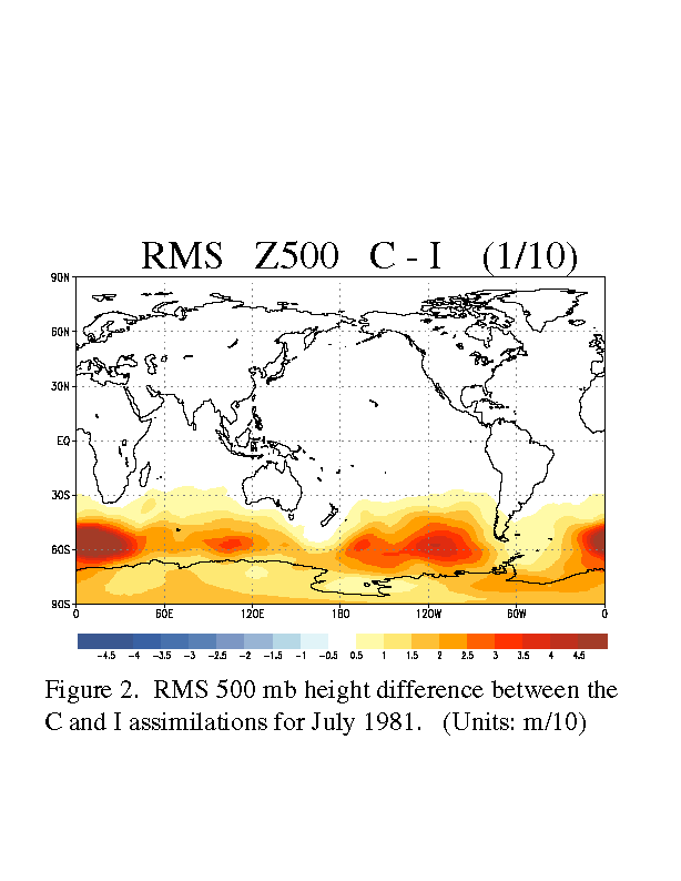
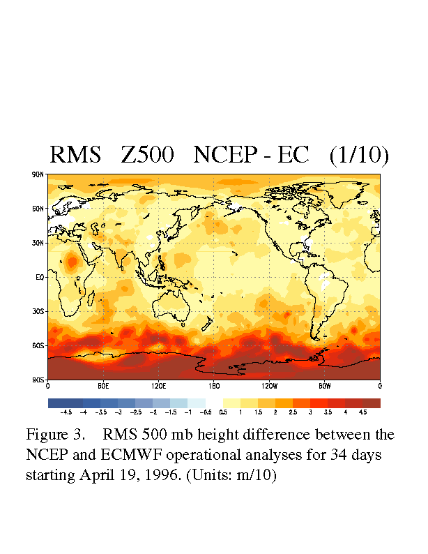
Differences between the C and I analyses were compared to differences between the NCEP and ECMWF operational analyses. The latter may be viewed as an additional measure of the analysis uncertainty. Ideally we would have compared ECMWF's Reanalysis against the C and I analyses but such data was unavailable. In addition the comparison between operational analyses was made for a different month but, nevertheless, should give a rough estimate of the analysis uncertainty. Figure 2 shows the RMS 500 mb height difference between the C and I analyses for July 1981. Equatorward of 30° S, the RMS difference is less than 5 meters. Peak values, in excess of 45 meters are found near 55° S. Figure 3 shows the RMS difference between the NCEP and ECMWF operational analyses for a 34 day period (April 19 - May 22, 1996). Comparison of Figs. 2 and 3 shows that equatorward of 30° S, the C and I analyses are much more similar than are the two operational analyses. Poleward of 30° S, the differences have similar magnitudes, though the C-I differences are largest over the southern oceans (and decrease towards the pole) while the NCEP-ECMWF differences increase towards the pole. As a caveat we note that Fig. 2 is based on analyses every 6-h while Fig. 3 is based on analyses every 12-h.
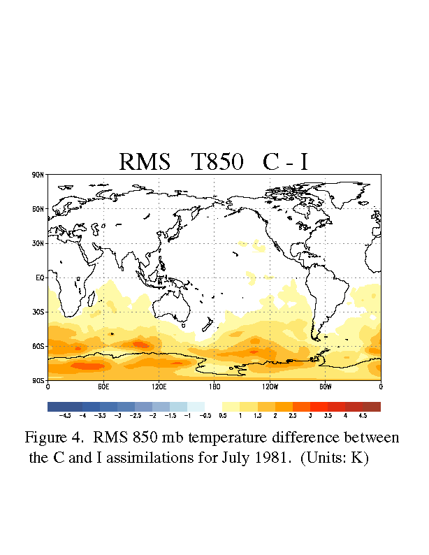
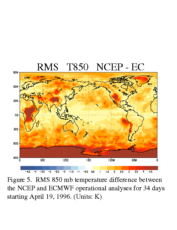
Figure 4 shows the RMS 850 mb temperature difference between the C and I assimilations for July 1981. Equatorward of 40° S, the RMS difference is less than 1 degree. For comparison, Fig. 5 shows the RMS difference between the NCEP and ECMWF operational analyses. Now we find that the difference between the C and I assimilations is less than the difference between the operational analyses.
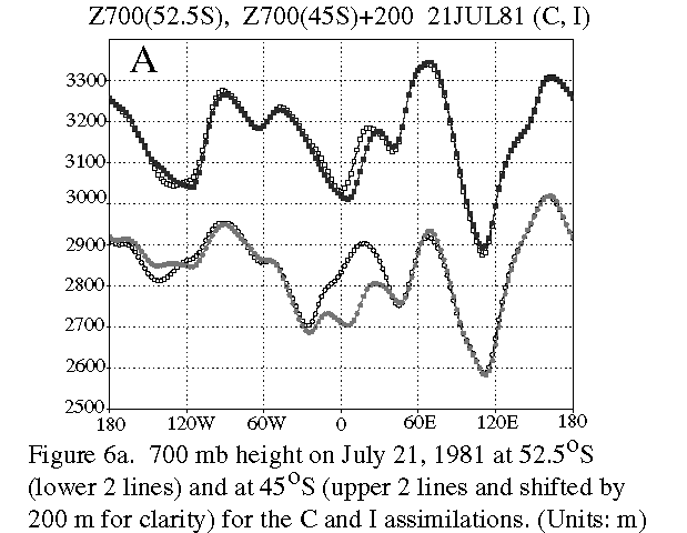
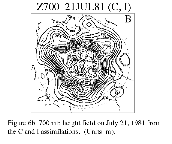
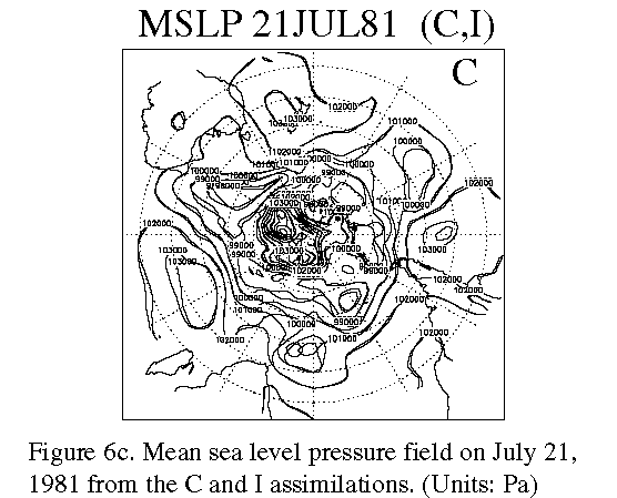
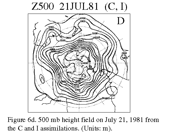
Figures 6a, 6b, 6cand 6d show the C and I analyses for 00Z on July 21, 1981. This date was chosen because the C and I analyses show large differences southwest of Africa (see the case study in section III below). Figure 6a shows that the 700 mb heights for the C and I analyses at 52.5° S (lower two lines) differ considerably in the vicinity of the Greenwich meridian. The upper two lines are the 700 mb heights (shifted by 200 m for clarity) at 45° S, which show smaller differences. Figure 6b shows the synoptic situation for Fig. 6a; clearly, the large-scale features are captured by both analyses, but there are regional differences (e.g. southwest of Africa) which also show up in mean SLP (Fig. 6c) and in the 500 mb heights (Fig. 6d). Overall, these results indicate that the PAOBS mislocation has little impact on global-scale / monthly mean features but does have impact on regional features at synoptic time scales (to be explored further in section III below).
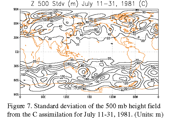
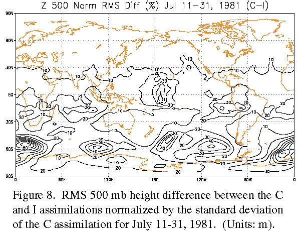
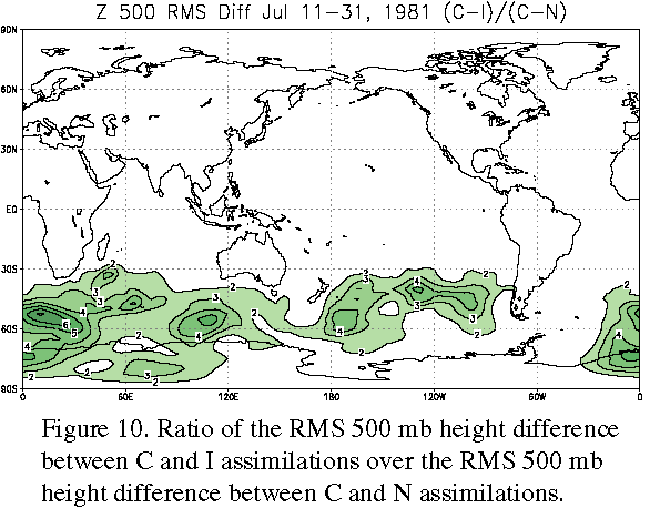
The impact of the PAOBS error on the variability in the SH mid-latitudes at diurnal (6-hourly) time scales is assessed in this section. Figure 7 shows the standard deviation of the 500 mb heights for the C assimilation; this plot includes the last 21 days of July 81 because the difference between the C and N experiments becomes small after about July 10. Figure 8 shows the RMS difference between the C and I assimilations normalized by the standard deviation of the C run (Fig. 7) for the same period; for reference the normalized RMS difference between the C and N experiments is shown in Fig. 9. Differences in excess of 0.5 standard deviations are found in C-I in the middle and high latitudes of the SH, particularly in the eastern ocean basins and over the storm tracks. Differences in C-N are located mainly in the tropics, where the variability is small. For convenience, we also show the ratio C-I/C-N, which gives the factor increase in the RMS difference (Fig. 10). We note that the results shown in these figures are typical of those found at lower levels and at the surface. These results suggest that studies of the statistics of the SH storm track at diurnal and daily time scales will be influenced by this additional source of uncertainty. While not shown, we note that similar results are obtained for other variance and covariance statistics.
Users of the SH Reanalysis may be tempted to do regional (i.e. synoptic-scale) case studies. Below we present an assessment of the impact of the PAOBS mislocation on a typical synoptic event. Figure 11 shows Hovmoeller (longitude- time) diagrams of the mid-latitude (40° S-50° S) surface pressure difference for C-I (Fig. 11a), C-N (Fig. 11b) and I-N (Fig. 11c) assimilations during July 1981 based on 6-hourly data. Figure 11a shows that sizable differences occur from time to time, primarily in the eastern ocean basins of the SH; further analysis of these events shows that they are usually linked to individual synoptic-scale features that are present in one assimilation but not the other, or that are shifted in amplitude and/or phase between assimilations.
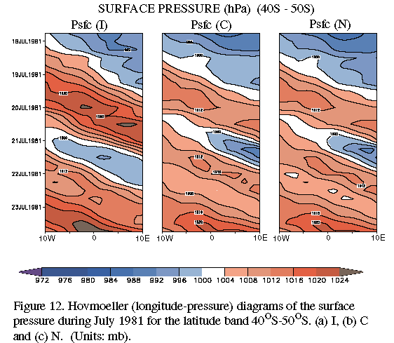
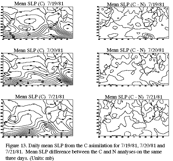
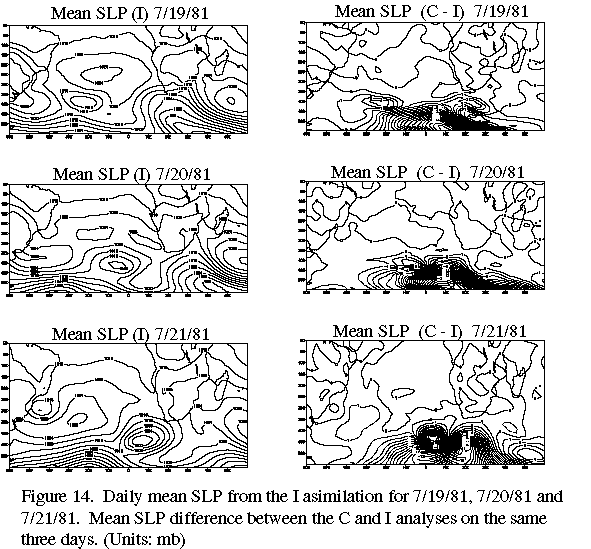
We now focus on a case that occurred around July 20, 1981 to the southwest of Africa (near the Greenwich Meridian). Examination of the surface pressure in mid-latitudes for this case (Fig. 12) shows sizable differences in amplitude and phase between the C and I runs. Spatial maps of the daily mean SLP during this period (Figs. 13a and 14a) show that these differences are linked to the evolution of a cyclone to the southwest of Africa. Comparisons to the original PAOBS data suggest that around the 18th of July mislocated PAOBS data were assimilated; this is clearly evident by July 19 from a comparison of the SLP field near 45° S, 10° W in the C (Fig. 13a) and I (Fig. 14a) runs. Differences between the C and I runs (Fig. 14b) are considerable and take on a characteristic dipole pattern seen in other case studies. As we move forward in time, these differences propagate towards the east around the southern tip of Africa. Where there is data to constrain the assimilation (i.e. over Africa) these errors do not grow. However, where there is little or no data (i.e. just south of Africa on 7/21) these errors persist and make their way into the western Pacific later in the month. Examination of vertical cross-sections of the height field at 45° S (Fig. 15) show that these errors are largest near the surface and tend to "propagate" upward in time reaching values in excess of 60 m at 500 mb. These values are typical of differences found in other case studies.
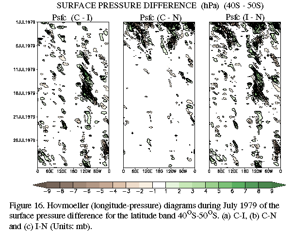
These results indicate that differences between the C and I runs for regional case studies can be larger than the analysis uncertainty. This appears to occur most often over the eastern oceans in the SH storm tracks. At very high southern latitudes (> 70° S), the impact of the PAOBS mislocation is smaller. These results imply that the tracking of storms over the middle and high latitudes of the SH at diurnal and daily time scales may be difficult. The difference fields in Fig. 14b are large enough to suggest that some subsequent "good" data might be rejected by the QC after the "bad" PAOBS data has been assimilated; this needs to be investigated. Moreover, comparison of July 1979 and July 1981 (compare Fig. 16 to Fig. 11) suggests that the relative influence of the PAOBS data is somewhat smaller during 1979, at least for regional studies. Finally, we note that many synoptic events show little or no impact of the PAOBS mislocation while others show a large impact; the reasons for this are not well understood. Additional assessments of the impact of the assimilation of the mislocated PAOBS and the subsequent influence on the assimilation are needed.
Figure 2. RMS 500 mb height difference between the C and I assimilations for July 1981. (Units: m/10)
Figure 3.RMS 500 mb height difference between the NCEP and ECMWF operational analyses for 34 days starting April 19, 1996. (Units: m/10)
Figure 4. RMS 850 mb temperature difference between the C and I assimilations for July 1981. (Units: K)
Figure 5. RMS 850 mb temperature difference between the NCEP and ECMWF operational analyses for 34 days starting April 19, 1996. (Units: K)
Figure 6. (a) 700 mb heights on July 21, 1981 at 52.5° S (lower 2 lines) and at 45° S (upper 2 lines and shifted by 200 m for clarity) for the C and I assimilations. Spatial maps of (b) the 700 mb height field, (c) the mean sea level pressure field and (d) the 500 mb height field on July 21, 1981 from the C and I assimilations.
Figure 7. Standard deviation of the 500 mb height field from the C assimilation for July 11-31, 1981. (Units: m)
Figure 8. RMS 500 mb height difference between the C and I assimilations normalized by the standard deviation of the C assimilation for July 11-31, 1981. (Units: m).
Figure 9. RMS 500 mb height difference between the C and N assimilations normalized by the standard deviation of the C assimilation for July 11-31, 1981. (Units: m).
Figure 10. Ratio of the RMS 500 mb height difference between C and I assimilations over the RMS 500 mb height difference between C and N assimilations.
Figure 11. Hovmoeller (longitude-pressure) diagrams during July 1981 of the surface pressure difference for the latitude band 40° S-50° S. (a) C-I, (b) C-N and (c) I-N (Units: mb).
Figure 12. Hovmoeller (longitude-pressure) diagrams of the surface pressure during July 1981 for the latitude band 40° S-50° S. (a) I, (b) C and (c) N. (Units: mb).
Figure 13. Daily mean SLP from the C assimilation for 7/19/81, 7/20/81 and 7/21/81. Mean SLP difference between the C and N analyses on the same three days. (Units: mb)
Figure 14. Daily mean SLP from the I assimilation for 7/19/81, 7/20/81 and 7/21/81. Mean SLP difference between the C and I analyses on the same three days. (Units: mb)
Figure 15. Longitude-height cross section of the height difference at 45° S between the C and I assimilations on 7/19/81, 7/20/81 and 7/21/81. (Units: m)
Figure 16. Hovmoeller (longitude-pressure) diagrams during July 1979 of the surface pressure
difference for the latitude band 40° S-50° S. (a) C-I, (b) C-N and (c) I-N (Units: mb).