[Previous Article] [Next Article]
Constructed Analogue Prediction of the East Central
Tropical Pacific SST through Winter 1998-99
contributed by Huug van den Dool
Climate Prediction Center, NOAA, Camp Springs, Maryland
Because excellent naturally occurring analogues are highly unlikely to occur, we may benefit from
constructing an analogue having greater similarity than the best natural analogue. As described in
Van den Dool (1994), the construction is a linear combination of observed anomaly patterns in
the predictor fields such that the combination is as close as desired to the base. Here, we forecast
the future SST anomaly in the ENSO-related east-central tropical Pacific ("Niño 3.4", or 5oN-5oS,
120-170oW). We use as our predictor (the analogue selection criterion) the first 5 EOFs of the
global SST field at four consecutive 3-month periods prior to forecast time. Predictor and
predictand data extending from 1955 to the present are used for a priori skill evaluation.
For any given base time (i.e. previous ones extending back to 1955, or the current "operational
forecast" ending with May 1997), a linear combination is made of the global SST patterns (using
the first 5 EOFs) from all 40 years (excluding the base year), so as to match the SST pattern of
the base time as closely as possible. This is done by classical least-squares multiple regression,
with each year's SST state as a predictor to which a weight is assigned, determined by inverting
the 40 X 40 (available years) covariance matrix. The weights assigned each year to reconstruct
the base SST state are then applied to the subsequently occurring Niño 3.4 SST in the predictand
period for these years, thereby constructing the forecast for the base year's predictand period.
Additional detail about the constructed analogue method is found in the September 1994 issue of
this Bulletin and in Van den Dool (1994). In the latter paper it is shown that constructed
analogues outperform natural analogues in specification mode (i.e. "forecasting" one
meteorological variable from another, contemporaneously). This advantage may be expected to
occur in actual forecasting also, as long as the (linear) construction does not compromise the
physics of the system too much. Brief discussion of the skill of the constructed analogue method
in forecasting SST is given in Van den Dool and Barnston (1995).
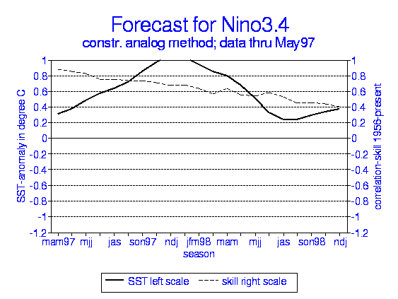
The forecasts for Niño 3.4 for 0 to about 1.5 years lead using constructed analogues are shown in
Fig. 1, using data through May 1997. The expected cross-validated skill is also shown. In Fig. 1
the SST anomaly observed during Mar-Apr-May 1997 is plotted as the earliest "forecast" value.
For Apr-May-Jun and May-Jun-Jul the observed SST for Dec-Jan-Feb enters into the plotted
forecast with a 2/3 and 1/3 weight, respectively, providing continuity with the known initial
condition.
A closer look at the skill of the constructed analogue method is provided by Fig. 2 in the June
1996 issue of this Bulletin (p. 73). The skill is competitive with those of other empirical as well as
dynamical methods (Barnston et al. 1994). Forecasts for late fall through winter tend to be most
skillful at short as well as long lead times, while summer forecasts have relatively lower skill.
While skill (dashed line in Fig. 1) generally decreases with lead time, the dependence on the target
season can sometimes be a stronger factor.
The presently above normal and increasing Niño 3.4 SST is forecast to warm further before
reaching a maximum anomaly of near +1.1oC toward the end of 1997. A return to near normal is
predicted by boreal summer of 1998.
Table 1 provides information about the role of each of the past years in the construction process
for the current forecasts. The inner product shows the degree of similarity (or, if negative,
dissimilarity) of this year's predictor periods to those of the other years. The weight shows the
contribution of each year's pattern to the constructed analogue. The inner products and the
weights, while similar, are not proportional. This is because, for example, two analogues having
the same kind of similarity are unnecessary; only one of them may have been assigned the
appropriately high weight, leaving the other with little to contribute.
The important positive (+) and negative (-) contributors to the description of the global SST over
the last 4 seasons (JJA 1996 to MAM 1997) are, in chronological order, 1964(-), 1966(-),
1973(-), 1976(-), 1981(+), 1989(+), 1990(+), and 1992(+). Some interdecadal variability in this
analogue time series is suggested by a tendency for temporal grouping of like-signs. More
negative than positive weights are found in the earlier ~60% of the record, and vice versa from
the late 1970s onward.
The result of the process is a forecast for a continuation of the warming already in evidence. In fact, the observations have "jumped the gun" on this forecast, having already attained approximately the levels predicted for the late fall. Thus, either the forecast will turn out to be too conservative, or the current rapid warming will level off (or even subside slightly) in the next few months, forming a short-term spike within a smoother low frequency time series that is more likely to be successfully modeled here using the first 5 EOFs of SST. Looking at some of the most influential years, we note that the by-far most strongly weighted year is negatively weighted (i.e. 1973, which denotes the period of June 1972 to May 1973). A warm event developed during 1972 and lasted through early 1973, switching to cold by late April 1973 and evolving into a strong cold event from fall 1973 to summer 1974. Of the four years having strong positive weights (1981, 89, 90 and 92), 1981 was relatively neutral with respect to ENSO, 1989 had been cold and then returned to near normal, 1990 had been slightly cold to neutral and then became somewhat warm, and 1992 unquestionably featured a warm event from spring 1991 through early summer 1992. We see that while there is some tendency for positive weights to be assigned to years in which cool or neutral SST was turning to warm SST (and vice versa for negative weights), processes other than ENSO also determine the weighting process and the resulting forecast. The weights shown in Table 1 suggest the existence of phenomena that vary on decadal or even longer time scales.Table 1. Inner products (IP; scaled such that sum of absolute values is 100) and weights (Wt; from multiple regression) of each of the years to construct an analogue to the sequence of 4 consecutive 3-month periods defined as the base (JJA and SON 1996, DJF 1996-97, and MAM 1997). Years are labeled by the middle month of the last of the four predictor seasons.
| Year | IP | Wt | Year | IP | Wt | Year | IP | Wt | Year | IP | Wt |
| 56 | -1 | 0 | 67 | -3 | -1 | 78 | -4 | -5 | 89 | 4 | 13 |
| 57 | 0 | 4 | 68 | -1 | 1 | 79 | -1 | 0 | 90 | 8 | 14 |
| 58 | 0 | 3 | 69 | 2 | 7 | 80 | 1 | 5 | 91 | 5 | 9 |
| 59 | -1 | -8 | 70 | 1 | 5 | 81 | 1 | 10 | 92 | 3 | 11 |
| 60 | 0 | 4 | 71 | -1 | -2 | 82 | 8 | 5 | 93 | 3 | 7 |
| 61 | -1 | 0 | 72 | -2 | -2 | 83 | 0 | -4 | 94 | 3 | -3 |
| 62 | -1 | -2 | 73 | -4 | -20 | 84 | 2 | -1 | 95 | 3 | 3 |
| 63 | 0 | 3 | 74 | -1 | 0 | 85 | 4 | 7 | |||
| 64 | -3 | -10 | 75 | -4 | -6 | 86 | 6 | 7 | |||
| 65 | 0 | 2 | 76 | -2 | -11 | 87 | 3 | 9 | |||
| 66 | -4 | -12 | 77 | -5 | -9 | 88 | 1 | -4 |
Barnston, A.G., H.M. van den Dool, S.E. Zebiak, T.P. Barnett, M. Ji, D.R. Rodenhuis, M.A.
Cane, A. Leetmaa, N.E. Graham, C.F. Ropelewski, V.E. Kousky, E.A. O'Lenic and R.E. Livezey,
1994: Long-lead seasonal forecasts--Where do we stand? Bull. Amer. Meteor. Soc., 75,
2097-2114.
van den Dool, H.M., 1994: Searching for analogues, how long must we wait? Tellus, 46A,
314-324.
van den Dool, H.M. and A.G. Barnston, 1995: Forecasts of global sea surface temperature out to
a year using the constructed analogue method. Proceed-ings of the 19th Annual Climate
Diagnostics Workshop, Nov. 14-18, 1994, College Park, Maryland, 416-419.
Fig. 1. Time series of constructed analogue forecasts (solid line) for Niño 3.4 SST based on the
sequence of four consecutive 3-month periods ending in May 1997. The dashed line indicates the
expected skill (correlation) based on historical performance for 1956-96. The x-axis represents the
target period. The verifying observation is shown instead of the constructed analogue
specification for Mar-Apr-May 1997, and this observation also contributes by decreasing amounts
to the Apr-May-Jun and May-Jun-Jul plotted values (see text).