Because excellent naturally occurring analogues are highly unlikely to occur, we may benefit from constructing an analogue having greater similarity than the best natural analogue. As described in Van den Dool (1994), the construction is a linear combination of observed anomaly patterns in the predictor fields such that the combination is as close as desired to the base. Here, we forecast the future SST anomaly in the ENSO-related east-central tropical Pacific ("Niño 3.4", or 5oN-5oS, 120-170oW). We use as our predictor (the analogue selection criterion) the first 5 EOFs of the global SST field at four consecutive 3-month periods prior to forecast time. Predictor and predictand data extending from 1955 to the present are used.
For any given base time (i.e. previous ones extending back to 1955, or the current "operational forecast" ending with February 1996), a linear combination is made of the global SST patterns (using the first 5 EOFs) from all 39 years (excluding the base year), so as to match the SST pattern of the base time as closely as possible. This is done by classical least-squares multiple regression, with each year's SST state as a predictor to which a weight is assigned, determined by inverting the 39 X 39 (available years) covariance matrix. The weights assigned each year to reconstruct the base SST state are then applied to the subsequently occurring Niño 3.4 SST in the predictand period for these years, thereby constructing the forecast for the base year's predictand period.
Additional detail about the constructed analogue method is found in the September 1994 issue of this Bulletin and in Van den Dool (1994). In the latter paper it is shown that constructed analogues outperform natural analogues in specification mode (i.e. "forecasting" one meteorological variable from another, contemporaneously). This advantage may be expected to occur in actual forecasting also, as long as the (linear) construction does not compromise the physics of the system too much. Brief discussion of the skill of the constructed analogue method in forecasting SST is given in Van den Dool and Barnston (1995).
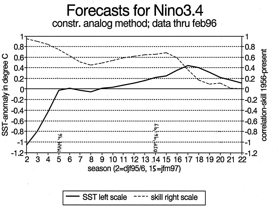
The forecasts for Niño 3.4 for 0 to about 1.5 years lead using constructed analogues are shown in Fig. 1, using data through February 1996. The expected cross-validated skill is also shown. The skill is competitive with those of other empirical as well as dynamical methods (Barnston et al. 1994). In Fig. 1 the SST anomaly observed during Dec-Jan-Feb 1995-96 is plotted as the earliest "forecast" value. For Jan-Feb-Mar and Feb-Mar-Apr the observed SST for Dec-Jan-Feb enters into the plotted forecast with a 2/3 and 1/3 weight, respectively, providing continuity with the known initial condition.
The present below normal SST conditions are forecast to dissipate by middle to late spring 1996, becoming slightly above normal from fall onward with a weak but broad peak centered in spring 1997. The specification for Dec-Jan-Feb (not shown) is only about a third of the observed negative anomaly. Reasons for this are likely similar to those which caused the same behavior three months ago, discussed in the December 1995 issue of this Bulletin. It was concluded that the most probable cause of the positive specification error is the uniqueness of the current SST developments.
Table 1 provides information about the role of each of the past years in the construction process for the current forecasts. The inner product shows the degree of similarity (or, if negative, dissimilarity) of this year's predictor periods to those of the other years. The weight shows the contribution of each year's pattern to the constructed analogue. The inner products and the weights, while similar, are not proportional. This is because, for example, two analogues having the same kind of similarity are unnecessary; only one of them may been assigned the appropriately high weight, leaving the other with little to contribute.
The important positive (+) and negative (-) contributors to the description of the global SST over the last 4 seasons (MAM 1995 to DJF 1995-96) are, in chronological order, 1966(-), 1973(-), 1976(-), 1983(-), 1986(+), 1988(+), 1989(+), 1990(+) and 1991(+). An interdecadal variability is suggested in this analogue time series, as a grouping of like-signs is evident. The weights are positive from 1984 to the present, suggesting that the present SST configuration is typical for the last 11 years and rather atypical for the years before 1984 except for 1956 and 1969-70.
The net result is a set of forecasts for a quick dissipation of the presently below normal Niño 3.4 SST, followed by a period of weak warmth from next fall through summer 1997. Looking at some of the strongly weighted years, we note that one of the positively weighted years was strongly cold (e.g. 1989, which denotes the period of Mar 1988 to Feb 1989), cold/neutral (1986), or neutral to neutral/warm (1990, 1991). However, 1988 was strongly warm and rapidly cooling. Three of the four strongly negatively weighted years were moderately to strongly warm (1966, 1973 and 1983); however, 1976 was clearly cold. While the weights are roughly similar to those shown for the constructed analogue forecast issued 3 months ago, this is the case to a lesser extent than usual. Negative weights are now assigned more clearly to warm episode years, and vice versa. Apparently the current cold period now occupies a sufficient portion of the 1-year set of predictor periods to match past cold (warm) episodes with fairly high (low) likelihood. That this does not occur as a "clean sweep", however, reminds us that phenomena other than ENSO are governing the weighting process. The weights shown in Table 1 suggest that one or more of such phenomena vary on decadal or still longer-term time scales.
Table 1. Inner products (IP; scaled such that sum of absolute values is 100) and weights (Wt; from multiple regression) of each of the years to construct an analogue to the sequence of 4 consecutive 3-month periods defined as the base (MAM 95, JJA 95, SON 95, and DJF 95-96). Years are labeled by the middle month of the last of the four predictor seasons.
Yr IP Wt Yr IP Wt Yr IP Wt56 -0 8 69 0 9 82 4 1
57 -3 -6 70 3 8 83 0 -10
58 -1 1 71 0 1 84 3 6
59 0 1 72 -4 -5 85 4 4
60 -1 4 73 -3 -10 86 4 10
61 -1 3 74 1 4 87 2 2
62 0 -1 75 -5 -7 88 3 10
63 1 5 76 -3 -12 89 4 14
64 0 -2 77 -5 -9 90 5 13
65 -3 -4 78 -6 -9 91 7 16
66 -5 -13 79 -4 -6 92 3 4
67 0 2 80 0 -2 93 2 2
68 -3 -4 81 2 1 94 3 5
Barnston, A.G., H.M. van den Dool, S.E. Zebiak, T.P. Barnett, M. Ji, D.R. Rodenhuis, M.A. Cane, A. Leetmaa, N.E. Graham, C.F. Ropelewski, V.E. Kousky, E.A. O'Lenic and R.E. Livezey, 1994: Long-lead seasonal forecasts--Where do we stand? Bull. Amer. Meteor. Soc., 75, 2097-2114.
van den Dool, H.M., 1994: Searching for analogues, how long must we wait? Tellus, 46A, 314-324.
van den Dool, H.M. and A.G. Barnston, 1995: Forecasts of global sea surface temperature out to a year using the constructed analogue method. Proceedings of the 19th Annual Climate Diagnostics Workshop, November 14-18, 1994, College Park, Maryland, 416-419.