[Previous Article] [Next Article]
Consolidated Forecasts of Tropical Pacific SST in Niño 3.4
Using Two Dynamical Models and Two Statistical Models
contributed by David Unger, Anthony Barnston, Huug van den Dool and Vern Kousky
Climate Prediction Center, NOAA, Camp Springs, Maryland
In this Bulletin we find a fairly large number of forecasts for the east-central tropical Pacific SST
for the coming year. Our objective here is to synthesize information from some of the predictive
sources into a single objective estimate of the likely evolution of the SST's in the tropical Pacific.
One approach to the problem is to combine, or consolidate, the forecasts of several models into a
single forecast. This could be done on the basis of the past behavior of each contributing model,
as well as the overlap of information among the models. There are several methods by which this
can be done. A common method, and the one used here, is linear multiple regression. In effect, a
statistical scheme is used to combine outputs of entire models whose natures themselves may be
statistical, dynamical, or a mixture of the two. In this case we use four input models. Two are
dynamical: the Lamont-Doherty (LD) Earth Observatory's simple coupled model, (the improved
LDEO2; Chen et al. 1995; Cane and Zebiak 1986), and the recently implemented CMP12 NCEP
coupled model (Ji et al. 1994). The other two models are statistical: the NCEP constructed
analogue (CA) model (Van den Dool 1994; Van den Dool and Barnston 1995), and the NCEP
canonical correlation analysis (CCA) model (Barnston 1994). The individual forecasts of each
model are shown elsewhere in this Bulletin issue.
To derive the multiple regression equations for each target season for each lead time, histories of
the forecasts of each model were obtained. The CCA and CA models have histories covering
1956-1996. The Lamont coupled model has a 1972-96 history, and the NCEP coupled model
1981-96. To circumvent the problem of the differing units and climatologies used, all forecasts
were converted to actual C forecasts. The observations were expressed likewise. The regressions
are based on forecasts for the Niño 3.4 region (5N-5S, 120-170W), except for the LD model,
from which we receive forecasts for the Niño 3 region. The Niño 3 forecast histories from the LD
model were used as a predictor for Niño 3.4 in the equation development. The regression
coefficients compensate for the slight differences between Niño 3 and Niño 3.4 to obtain the least
squares fit for Niño 3.4. We expect to begin receiving gridded forecast fields from Lamont
shortly, and will then be able to use Lamont's Niño 3.4 forecasts directly.
The desired lead times of the consolidated forecasts range from 0.5 months to 12.5 months by 1
month increments, where lead time is defined as the time skipped between the time of the forecast
and the beginning of the forecasted (target) period. For example, the forecasts shown here, which
are issued in the middle of March 1997, have target periods including Apr-May-Jun 1997,
May-Jun-Jul 1997,..., Apr-May-Jun 1998. Three of the four individual models have forecast
histories whose leads range to 12.5 months or greater, while one (the NCEP coupled model) has a
maximum lead of only 8.5 months. Consolidated forecasts for lead times higher than 8.5 months,
therefore, are based only on the other three models. A temporal smoother has been applied to the
forecasts to avoid any discontinuity in the forecast time series, however, a noticeable increase in
the error estimates occurs when the NCEP model drops from the consolidation.
Because the NCEP coupled model forecast only has a 1981-96 history, the training period for the
regression is limited to that period and thus results in greater uncertainty in the coefficients than
would be the case if a longer history could be used. When that model is not included in the
consolidation process for the longer lead times, the 1972-96 period is used to derive the
regression equations, making for a more favorable training sample. Data from three lead times
were pooled together to help equation stability and help smooth forecasts from projection to
projection. Predictor and predictand data from the season preceding and following the target
season were combined to form the regression equation. The first (last) target season shares the
equation with the adjacent season.
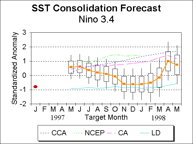
The consolidated forecast for Niño 3.4 made in mid-March 1997 is shown in Fig. 1. Forecasts
are expressed as standardized anomalies relative to the 1961-1990 climatology. The box and
whisker intervals for the forecasts indicate the one and two error standard deviations, based on
estimated skill following shrinkage of the dependent sample skill results in accordance with the
sample size and number of predictors. The compo-nent forecasts are displayed on the same chart
for comparison. Note that the LD anomalies are for Niño 3. The observed SST anomaly for the
most recent 3-mo period is also shown.
Three of the four models indicate rapid warming to well above normal conditions by AMJ 1997 followed by a slow increase thereafter, while one, the LD model, remains cold throughout the forecast. The wide dis-agreement among forecast models produces some undesirable characteristics in the time continuity of the consolidation forecast. The cosolidation forecast shows warming from the intital observation, to moderately above normal, by AMJ followed by a gradual cooling to moderately below normal SST's by late 1997, with a rapid warming in spring 1998. This time evolution is, in fact, not indicated by any of the componant models, and is a result of the statistical strength of each model as a function of lead time and target season.
The regression procedure favors the CCA, CA and NCEP solutions in the early leads. This is
partially because they use observed data through much of February, while the LD model uses data
only through January, 1997 in its forecast. The SST's in the tropical Pacific have warmed
considerably in the past two months, which is not reflected in the LD model. The consolidation
forecast places little weight on the LD model in the early projections, since its use of less current
initial data is reflected by lower skill on the historical forecasts when compared to the other
models. The LD model, however, is the most skillful model at longer leads for this initial time,
hence it receives more weight as the forecast progresses. At very long leads, the skill of all
models is low and the consolidation forecast approaches a simple mean of the components.
Combined, this produces an apparent trend in SST's which may appear to be unrealistic.
In view of its skill, the LD model cannot simply be dismissed at long leads. However, because
the recent warming in the observed Niño 3 region SST's is not reflected in the LD model's
forecast, the confidence in the forecast cold temperatures might be reduced somewhat, favoring a
more level trend, with temp-eratures remaining near normal through most of the forecast period
followed by warming in 1998.
The expected forecast error for this season is quite high, reflecting the so-called spring barrier
noted in SST predictions in the ENSO region. Even for the short leads the error bars are quite
wide. The accuracy of the forecast for next winter will increase considerably in the next few
months, once early summer SST patterns become established in the equatorial Pacific.
Acknowledgments: We are grateful to Stephen Zebiak and Mark Cane of Lamont Doherty Earth
Observatory, and Ming Ji and Ants Leetmaa from the National Centers for Environmental
Prediction, for providing the forecast histories from their respective dynamical models, as well
as their current real-time forecasts.
Barnston, A.G., 1994: Linear statistical short-term climate predictive skill in the Northern
Hemisphere. J. Climate, 5, 1514-1564.
Cane, M., S.E. Zebiak and S.C. Dolan, 1986: Experimental forecasts of El Niño. Nature, 321,
827-832.
Chen, D., S.E. Zebiak, A.J. Busalacchi and M.A. Cane, 1995: An improved procedure for El Niño
forecasting: Implications for predictability. Science, 269, 1699-1702.
Ji, M., A. Kumar and A. Leetmaa, 1994: An experimental coupled forecast system at the
National Meteorological Center: Some early results. Tellus, 46A, 398-418.
van den Dool, H.M., 1994: Searching for analogues, how long must we wait? Tellus, 46A,
314-324.
van den Dool, H.M. and A.G. Barnston, 1995: Forecasts of global sea surface temperature out to
a year using the constructed analogue method. Proceedings of the 19th Annual Climate
Diagnostics Workshop, November 14-18, 1994, College Park, Maryland, 416-419.
Fig. 1. Consolidated forecast (thick line) for the standardized anomaly of the SST in the Niño
3.4 region (5N-5S, 120-170W) for the next 13-running 3-month periods. Month labels on the
abscissa denote the middle months of the 3-month predictand period. Box and whiskers for each
point indicate the one and two error standard deviation intervals. The latest observation
(Dec-Jan-Feb 1996/97) is also shown by the filled ellipse. The prediction from each component
model is shown for comparison.