[Previous Article]
[Next Article]
Forecast of PacificŁIndian Ocean SSTs Using
Linear Inverse Modeling
contributed by Cecile Penland1, Klaus Weickmann2
and Catherine Smith1
1CIRES, University of Colorado, Boulder, Colorado
2Climate Diagnostics Center (CDC),
ERL/NOAA, Boulder, Colorado
Using the methods described in Penland and Magorian (1993)
and in previous issues of this Bulletin (particularly the December 1992
and June 1993 issues), the pattern of IndoPacific sea-surface temperature
anomalies (SSTAs), the SSTA in the Nino 3 region (6oNŁ6oS,
90 oŁ150 oW), and the SSTA in the Nino 4 region (6oNŁ6oS,
150 oW-160 oE) are predicted. A prediction at lead
time t is made by applying a statistically-obtained Green function
G(t) to an observed initial condition consisting of SST anomalies
(SSTAs) in the IndoPacific basin. Three-month running means of the temperature
anomalies are used, the seasonal cycle has been removed, and the data have
been projected onto the 20 leading empirical orthogonal functions (EOFs)
explaining about 73% of the variance. The Nino 3 region has an RMS temperature
anomaly of about 0.7oC; the inverse modeling prediction method
has an RMS error of about 0.5oC at a lead time of nine months
and approaches the RMS value at lead times of 18 months to two years. The
COADS 1950-79 climatological annual cycle has been removed.
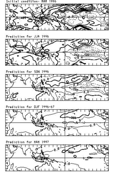
The predicted IndoPacific SSTA patterns based on the Mar-Apr-May
1996 initial condition for the following Jun-Jul-Aug, Sep-Oct-Nov, Dec-Jan-Feb
1996-97 and Mar-Apr-May 1997 are shown in Fig. 1 (contour interval is 0.2oC).
Figure 2a shows the predictions (light solid or dotted lines) of the NiZo
3 anomaly for initial conditions Dec-Jan-Feb 1995-96, Jan-Feb-Mar, Feb-Mar-Apr
and Mar-Apr-May 1996. Dashed lines indicate the 1 standard deviation expected
error for the prediction based on the Dec-Jan-Feb initial conditions. Predictions
based on Dec-Jan-Feb 1995-96 and Mar-Apr-May 1996 initial conditions are
indicated by arrows in the graphs. Figure 2b is the same, but for the NiZo
4 region. Verifications consisting of contributions to the appropriate
region by the 20 leading EOFs (heavy dashed line) and those including the
truncation error (heavy solid line) are also shown.
The initial condition in Fig. 1 is not much different
from the 3-month forecast published in the March issue of this Bulletin
with one major exception: SSTAs in the far eastern south tropical Pacific
(70-90EW, 2-26ES) are colder than predicted. We believe this to be a consequence
of a transition to strong southeasterly trades there which occurred in
April. This event appears to have affected a key area of the predictor
region so that the forecast for the rest of this year is for continued
cool, or even colder, SSTAs in the eastern tropical Pacific rather than
the warm anomalies previously forecast.
Penland, C. and T. Magorian, 1993: Prediction of NiZo
3 seaŁsurface temperatures using linear inverseŁ modeling. J. Climate,
6, 1067Ł1076.
Fig. 1. Linear inverse modeling forecasts of SST
anomalies, relative to the standard 1950-79 COADS climatology both for
the training period (1950-84) and for these forecasts. Forecast anomalies
are projected onto 20 leading EOFs, based on Mar-Apr-May 1996 initial conditions
(top panel). Contour interval is 0.2oC. Positive anomalies are
represented by heavy solid lines, negative anomalies by dashed lines. SST
anomaly data have been provided by NCEP, courtesy of R.W. Reynolds. Prediction
by linear inverse modeling is described in Penland and Magorian (1993).
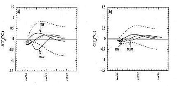
Fig. 2 (a): Inverse modeling predictions (light
solid or dotted lines) of NiZo 3 SSTA for initial conditions Dec-Jan-Feb
1995-96, Jan-Feb-Mar, Feb-Mar-Apr and Mar-Apr-May 1996. Dashed lines indicate
the 1 standard deviation expected error for the Dec-Jan-Feb prediction.
Heavy dashed line indicates the contribution to the verification from the
20 leading EOFs; the heavy solid line indicates the verification including
the truncation error. (b): As in (a) except for Nino 4. Prediction by linear
inverse modeling is described in Penland and Magorian (1993).