A neural network model has been developed for forecasting the tropical Pacific SST in the Nino 3 region. Based on our earlier neural network models (Tang et al. 1994; Tangang et al. 1996), this current model has a number of new techniques added to better deal with noisy data, mainly the additional continuity term and the Aclearning@ term in the cost function. The word Aclearning@ is derived from Alearning@ and Acleaning@, meaning that the neural network learns from the data and cleans the data at the same time (Weigend et al. 1996). In the March 1996 issue of this Bulletin, the detail of this model was described, and the hindcast and retrospective forecast skills were given.

The data used for training are the NiZo 3 SST index and the first 4 EOF coefficients of the FSU monthly wind stress data (Goldenberg and O'Brien 1981). The seasonal cycle, calculated from the 1961-90 data, has been removed from the NiZo 3 data. Before the EOF calculation, the wind data were first smoothed with one pass of a 1­2­1 filter in zonal and meridional directions and in time, and detrended and de­seasoned by subtracting from a given month the average of the same calendar months of the previous four years. This pre­EOF processing is the same as that used in Lamont's coupled model (Cane et al. 1986) and in Tang (1995).

The inputs of the neural network for a given month consist of the NiZo 3 index and the first 4 wind EOF coefficients of the month and the same 5 numbers for the month that is 3 months earlier, amounting to 10 inputs to the network. These inputs feed into a hidden layer with 4 sigmoidal neurons, which in turn feed into 5 linear output neurons, giving the NiZo 3 and the first 4 wind EOF coefficients for the month that is 3 months later. Thus, the time step of the neural network is 3 months. By repeatedly applying the model output as input to the neural network, we can obtain forecasts for longer lead times. There are 420 training pairs (i.e., sets of predictors and predictands) in the 1961-95 period.

To estimate the forecast skill, retroactive real time forecasts 1986-1995 were carried out. Figures 1 and 2 of the March 1996 issue of this Bulletin show the skill in terms of correlation and RMS error for retroactive real time as well as hindcasts for a longer historical period. Skills are seen to be competitive with other empirical forecast approaches such as analogs or linear regression.

The model we use here is the same as the one we used in the last issue of this Bulletin. However, the initial conditions have been adjusted with the new data using the same optimization as the model training, in a way similar to initialization of adjoint data assimilation.

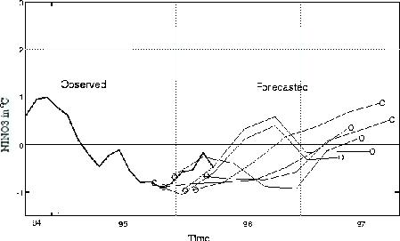
Figure 1 shows the latest forecast using a neural network trained with data up to April 1996. Six forecasts of lead times of up to 18 months were initiated from October to March 1996. Our forecast calls for a normal, or a slightly cool tropical condition in the 1996-97 boreal winter. We caution that our forecasts using data up to February 1996 called for a warm 1996-97 winter; now with the March and April data added, the forecasts became cooler.

The forecast of our neural network model is updated monthly in our web site. In addition, our web site issues forecasts by a POP model (Tang 1995). The POP model forecasts the continuation of the current cold condition for the coming season, but has not called for any warm or cold event for the 1996-97 winter so far.

Cane, M.A., S.E. Zebiak and S. Dolan, 1986: Experimental forecasts of El Nino. Nature, 321, 827­832.

Goldenberg, S.B., and J.J. O'Brien, 1981: Time and space variability of tropical Pacific wind stress. Mon. Wea. Rev., 109, 1190­1207.

Tang, B., 1995: Periods of linear development of the ENSO cycle and POP forecast experiments. J. Climate, 8, 682­691.

Tang, B.,G. Flato and G. Holloway, 1994: A study of Arctic sea ice and sea level pressure using POP and neural network methods. Atmos.­Ocean, 32, 507­529.

Tangang, F.T., W.W. Hsieh and B. Tang, 1996: Forecasting the equatorial Pacific see surface temperatures by neural network models. Climate Dynamics, accepted.

Weigend, A.S, H.G. Zimmermann, and R. Neuneier, 1996: Clearning. In Neural Networks in Financial Engineering. Refenes, P., Y. Abu-Mostafa, J.E. Moody and A.S. Weigend, Eds. Proceedings, Neural Networks in the Capital Markets, October 1995, London, UK. In press.

Figures