Because excellent naturally occurring analogues are highly unlikely to occur, we may benefit from constructing an analogue having greater similarity than the best natural analogue. As described in Van den Dool (1994), the construction is a linear combination of observed anomaly patterns in the predictor fields such that the combination is as close as desired to the base. Here, we forecast the future SST anomaly in the ENSO­related east­central tropical Pacific (ANiZo 3.4", or 5^oN­5^oS, 120­170^oW). We use as our predictor (the analogue selection criterion) the first 5 EOFs of the global SST field at four consecutive 3­month periods prior to forecast time. Predictor and predictand data extending from 1955 to the present are used for a priori skill evaluation.

For any given base time (i.e. previous ones extending back to 1955, or the current "operational forecast" ending with May 1996), a linear combination is made of the global SST patterns (using the first 5 EOFs) from all 39 years (excluding the base year), so as to match the SST pattern of the base time as closely as possible. This is done by classical least­squares multiple regression, with each year's SST state as a predictor to which a weight is assigned, determined by inverting the 39 X 39 (available years) covariance matrix. The weights assigned each year to reconstruct the base SST state are then applied to the subsequently occurring NiZo 3.4 SST in the predictand period for these years, thereby constructing the forecast for the base year's predictand period.

Additional detail about the constructed analogue method is found in the September 1994 issue of this Bulletin and in Van den Dool (1994). In the latter paper it is shown that constructed analogues outperform natural analogues in specification mode (i.e. "forecasting" one meteorological variable from another, contemporaneously). This advantage may be expected to occur in actual forecasting also, as long as the (linear) construction does not compromise the physics of the system too much. Brief discussion of the skill of the constructed analogue method in forecasting SST is given in Van den Dool and Barnston (1995).

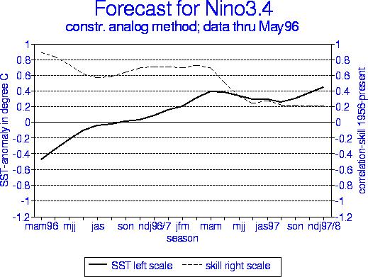
The forecasts for NiZo 3.4 for 0 to about 1.5 years lead using constructed analogues are shown in Fig. 1, using data through May 1996. The expected cross-validated skill is also shown. In Fig. 1 the SST anomaly observed during March-April-May 1996 is plotted as the earliest Aforecast@ value. For Apr-May-Jun and May-Jun-Jul the observed SST for Dec-Jan-Feb enters into the plotted forecast with a 2/3 and 1/3 weight, respectively, providing continuity with the known initial condition.

A more comprehensive examination of the skill is enabled by Fig. 2, where skill is shown as a function of the season in which the forecast is made (starting season; horizontal axis) and the lead time (vertical axis). The target season, while not explicitly shown, can be inferred by increasing the starting season by the lead time and adding another 3 months because of our definition of lead time. (Zero lead denotes a forecast for a 3-month period centered 3 months later than the centered starting season.) The skill is competitive with those of other empirical as well as dynamical methods (Barnston et al. 1994). Forecasts for late fall through winter tend to be most skillful at short as well as long lead times, while summer forecasts have relatively lower skill. While skill (dashed line in Fig. 1) generally decreases with lead time, the dependence on the target season can sometimes be a stronger factor, as seen in the apparent Areturn of skill@ from Jul-Aug-Sep 1996 to Feb-Mar-Apr 1997 in the current forecast (Fig. 1). Forecast skill as a function of lead when Mar-Apr-May is the starting season can be read also in Fig. 2 along the vertical line starting at the bottom at season=4.

The presently still slightly below normal SST conditions are forecast to return to normal by this summer and fall, becoming slightly warm by winter 1996-97 and especially spring 1997.

Table 1 provides information about the role of each of the past years in the construction process for the current forecasts. The inner product shows the degree of similarity (or, if negative, dissimilarity) of this year's predictor periods to those of the other years. The weight shows the contribution of each year's pattern to the constructed analogue. The inner products and the weights, while similar, are not proportional. This is because, for example, two analogues having the same kind of similarity are unnecessary; only one of them may have been assigned the appropriately high weight, leaving the other with little to contribute.

The important positive (+) and negative (-) contributors to the description of the global SST over the last 4 seasons (JJA 1995 to MAM 1996) are, in chronological order, 1966(-), 1973(-), 1976(-), 1977(-), 1984(+), 1988(+), 1989(+), and 1991(+). An interdecadal variability in this analogue time series is suggested by the temporal grouping of like-signs. The weights have been positive from 1984 to the present, suggesting that the present SST configuration is typical for the last 11 years and atypical for certain groups of years before 1984 such as the mid-1960s and most of the 1970s.

The result of the process is a set of forecasts for continued trend toward near normal SST followed by weak warmth for the first half of 1997. Looking at some of the strongly weighted years, we note that one of the positively weighted years was strongly cold (e.g. 1989, which denotes the period of June 1988 to May 1989), somewhat cold (1984), or neutral to neutral/warm (1991). However, 1988 was strongly warm and rapidly cooling. Three of the four strongly negatively weighted years were moderately to strongly warm (1966, 1973 and 1977); however, 1976 was decisively cold. We see that negative weights tend to be assigned to warm episode years, and vice versa. The mild cold period that is now concluding is well contained in the 1-year set of predictor periods, projecting positively (negatively) on past cold (warm) episodes. That this does not occur unfailingly, however, demonstrates that phenomena other than ENSO are governing the weighting process. The weights shown in Table 1 suggest that one or more of such phenomena vary on decadal or still longer-term time scales.

Table 1. Inner products (IP; scaled such that sum of absolute values is 100) and weights (Wt; from multiple regression) of each of the years to construct an analogue to the sequence of 4 consecutive 3-month periods defined as the base (JJA 95, SON 95, DJF 95-96, and MAM 96). Years are labeled by the middle month of the last of the four predictor seasons.

Barnston, A.G., H.M. van den Dool, S.E. Zebiak, T.P. Barnett, M. Ji, D.R. Rodenhuis, M.A. Cane, A. Leetmaa, N.E. Graham, C.F. Ropelewski, V.E. Kousky, E.A. O'Lenic and R.E. Livezey, 1994: Long­lead seasonal forecasts--Where do we stand? Bull. Amer. Meteor. Soc., 75, 2097-2114.

van den Dool, H.M., 1994: Searching for analogues, how long must we wait? Tellus, 46A, 314­324.

van den Dool, H.M. and A.G. Barnston, 1995: Forecasts of global sea surface temperature out to a year using the constructed analogue method. Proceedings of the 19th Annual Climate Diagnostics Workshop, November 14-18, 1994, College Park, Maryland, 416-419.

Fig. 1. Time series of constructed analogue forecasts (solid line) based on the sequence of four consecutive 3-month periods ending in May 1996. The dashed line indicates the expected skill (correlation) based on historical performance for 1956-95. The x-axis represents the target period. The verifying observation is shown instead of the constructed analogue specification for Mar-Apr-May 1996, and this observation also contributes by decreasing amounts to the Apr-May-Jun and May-Jun-Jul plotted values (see text).

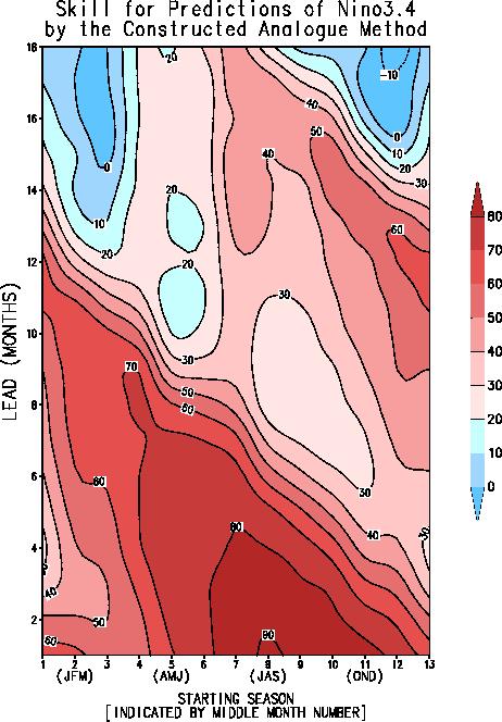
Fig. 2. Lead time versus starting season contour plot of constructed analogue skill (correlation X100) in predicting 3-month mean NiZo 3.4 SST anomaly using the evolution of global SST over the previous year as the analogue matching criterion. The horizontal axis denotes the forecast starting season (not the target season), and the vertical axis the lead time in months, where 0 is defined as a forecast whose target period begins at the time of the forecast.