In this Bulletin we find a fairly large number of forecasts for the east-central tropical Pacific SST for the coming year. Some predict continuation of the current cool episode throughout 1996. Others forecast a rapid dissipation, followed by varying degrees of warming as boreal winter 1996-97 approaches. The direction of the forecast is not related to the type of model--either statistical or dynamical models may go either way. Which models are we to believe this time, or any time?

One approach to the problem is to combine, or consolidate, the forecasts of several models into a single forecast. This could be done on the basis of the past behavior of each contributing model, as well as the overlap of information among the models. There are several methods by which this can be done. A common method, and the one used here, is linear multiple regression. In effect, a statistical scheme is used to combine outputs of entire models whose natures themselves may be statistical, dynamical, or a mixture of the two. In this case we use four input models. Two are dynamical: the Lamont-Doherty Earth Observatory=s simple coupled model (the improved LDEO2; Chen et al. 1995; Cane and Zebiak 1986), and the NCEP coupled model (Ji et al. 1994). The other two models are statistical: the NCEP constructed analogue (CA) model (Van den Dool 1994; Van den Dool and Barnston 1995), and the NCEP canonical correlation analysis (CCA) model (Barnston 1994). The individual forecasts of each model are shown elsewhere in this Bulletin issue.

To derive the multiple regression equations for each target season for each lead time, histories of the forecasts of each model were obtained. The CCA and CA models have histories covering 1956-1995. The Lamont coupled model has a 1972-95 history, and the NCEP coupled model 1982-95. To circumvent the problem of the differing units and climatologies used, all forecasts were converted to actual EC forecasts. The observations were expressed likewise. The regressions are based on forecasts for the NiZo 3.4 region (5EN-5ES, 120-170EW), except for the Lamont model, from which we receive forecasts for the NiZo 3 region. The Nino 3 forecast histories from the Lamont model were used as a predictor for NiZo 3.4 in the equation development. The regression coefficients compensate for the slight differences between NiZo 3 and Nino 3.4 to obtain the least squares fit for NiZo 3.4. We expect to begin receiving gridded forecast fields from Lamont shortly, and will then be able to use Lamont=s NiZo 3.4 forecasts directly.

The desired lead times of the consolidated forecasts range from 0.5 months to 11.5 months by 1 month increments, where lead time is defined as the time skipped between the time of the forecast and the beginning of the forecasted (target) period. For example, the forecasts shown here, which are issued in the middle of June 1996, have target periods including Jul-Aug-Sep 1996, Aug-Sep-Oct 1996, ..., Jun-Jul-Aug 1997. Three of the four individual models have forecast histories whose leads range to 11.5 months or greater, while one (the NCEP coupled model) has a maximum lead of only 7.5 months. Consolidated forecasts for lead times higher than 7.5 months, therefore, are based only on the other three models; a slight discontinuity in the forecast time series may thus be expected between the Feb-Mar-Apr and the Mar-Apr-May 1997 forecasts.

Because the NCEP coupled model forecast only has a 1982-95 history, the training period for the regression is limited to that period and thus results in greater uncertainty in the coefficients than would be the case if a longer history could be used. When that model is not included in the consolidation process for the longer lead times, the 1972-95 period is used to derive the regression equations, making for a more favorable training sample. Data from three lead times were pooled together to help equation stability and help smooth forecasts from projection to projection. Predictor and predictand data from the season preceding and following the target season were combined to form the regression equation. The first (last) target season shares the equation with the adjacent season.

An examination of the equation coefficients revealed that the sample size of only 14 years was insufficient to produce stable coefficients when all 4 models were included as predictors, since forecasts were stratified by season. Upon introduction of the fourth model, the two statistical models, CA and CCA, began to show evidence of multicollinearity, with regression coefficients of large magnitudes and opposite signs. The equation performance was greatly enhanced when the information from these two models was first combined into a single predictor by the use of a simple average of the two forecasts.

The consolidation forecast presented here uses NCEP, Lamont (Called ACZ@), and the mean of CCA and CA for predictors. The mean value of CCA and CA was also used as a predictor for lead times beyond 7.5 months when the consolidation no longer involved the NCEP model. There was very little difference on dependent data between forecasts produced from equations that used CZ, CA and CCA as predictors, and those that used CZ and the mean of the two statistical forecasts. The mean of CCA and CA was used for consistency with equations from earlier lead times.

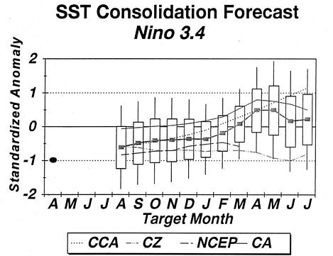
The consolidated forecast for NiZo 3.4 resulting from the multiple regression run in mid-June 1996, expressed as a standardized anomaly, is shown in Fig. 1. The box and whisker intervals for the forecasts at each time indicate the one and two error standard deviation, based on estimated skill following shrinkage of the dependent sample skill results in accordance with the sample size and number of predictors. The component forecasts are displayed on the same chart for comparison. Note that the CZ anomalies are for NiZo 3. The observed SST anomaly for the most recent 3-mo period is also shown.

The consolidation forecast remains at about a half of a standard deviation below normal through the remainder of 1996, followed by a fairly rapid warming to nearly a half standard deviation above normal by Mar-Apr-May 1997. The warming was not simply the result of the loss of the NCEP model in the regression weighting, since the predicted warming was well underway the before the NCEP model=s final projection.

Acknowledgments: We are grateful to Stephen Zebiak and Mark Cane of Lamont Doherty Earth Observatory, and Ming Ji and Ants Leetmaa from the National Centers for Environmental Prediction, for providing the forecast histories from their respective dynamical models, as well as their current real-time forecasts.

Barnston, A.G., 1994: Linear statistical short-term climate predictive skill in the Northern Hemisphere. J. Climate, 5, 1514-1564.

Cane, M., S.E. Zebiak and S.C. Dolan, 1986: Experimental forecasts of El Nino. Nature, 321, 827­832.

Chen, D., S.E. Zebiak, A.J. Busalacchi and M.A. Cane, 1995:An improved procedure for El Nino forecasting: Implications for predictability. Science, 269, 1699-1702.

Ji, M., A. Kumar and A. Leetmaa, 1994: An experimental coupled forecast system at the National Meteorological Center: Some early results. Tellus, 46A, 398-418.

van den Dool, H.M., 1994: Searching for analogues, how long must we wait? Tellus, 46A, 314­324.

van den Dool, H.M. and A.G. Barnston, 1995: Forecasts of global sea surface temperature out to a year using the constructed analogue method. Proceedings of the 19th Annual Climate Diagnostics Workshop, November 14-18, 1994, College Park, Maryland, 416-419.