[Next Article] -
[Previous Article]
Forecasts of Tropical Pacific SST Using a Data
Assimilating Neural Network Model
contributed by Benyang Tang, William Hsieh and Fred Tangang
Department of Earth and Ocean Sciences, University of British Columbia, Vancouver, B.C., Canada
Web site of the UBC Climate Prediction Group:
http://www.ocgy.ubc.ca
A neural network model has been developed for
forecasting the tropical Pacific SST in the Niño 3
region. Based on our earlier neural network models
(Tang et al. 1994; Tangang et al. 1996), this current
model has a number of new techniques added to better
deal with noisy data.
Normally, when a neural network is trained, only
the network weights are adjusted to minimize a cost
function which measures only the differences between
the network output and the data. In our data
assimilating neural network, not only the weights, but
also the network input are adjusted. The cost function
to be minimized consists of three terms. The first term
is the cost function of a traditional neural network,
measuring the difference between the network output
and the data (the output constraint). This is simply the
error of the prediction. The second term measures the
difference between the network input and the raw data
(the input constraint). It was proposed by Weigend et al
(1996), and was termed "clearning", after the words
"learning" and "cleaning", meaning that the neural
network learns from the data and cleans the data at the
same time. Thus, the data are modified each time a
training cycle is performed, based on the assumption
that the raw predictor data contain some errors.
"Clearning" makes the input data more compatible with
the model, alleviating "transient growth" (Blumenthal
1991), somewhat similar to normal mode initialization
reducing initial gravity wave propagation with primitive
equations in numerical weather prediction. The third
term measures the difference between the network
output and the network input for the next step. It acts as
a weak constraint of continuity, forcing the end of one
step to be close to the beginning of the next step. This
term is usually smaller than the first and second terms,
as the first two involve the noisy raw data and the third
term contains only the smoothed model input and
output. During training, the input for each step is the
raw input data (first training cycle) or the cleaned data
(from "clearning", for subsequent training cycles).
When training is finished, the forecast starts from the
network output for the starting month obtained in the
training, instead of from the raw data, similar to
initialization by adjoint data assimilation. In a
forecasting exercise, each step is not a separate entity as
in a training cycle--rather, it is a multiple-step
application of the trained neural network, with no
exposure to the raw or cleaned data between steps.
The data used for training are the Nino 3 SST
index and the first 4 EOF coefficients of the FSU
monthly wind stress data (Goldenberg and O'Brien
1981). The seasonal cycle, calculated from the 1961-90
data, has been removed from the Niño 3 data. Before
the EOF calculation, the wind data were first smoothed
with one pass of a 1-2-1 filter in zonal and meridional
directions and in time, and detrended and de-seasoned
by subtracting from a given month the average of the
same calendar months of the previous four years. This
pre-EOF processing is the same as that used in
Lamont's coupled model (Cane et al. 1986) and in Tang
(1995).
The inputs of the neural network for a given
month consist of the Niño 3 index and the first 4 wind
EOF coefficients of the month and the same 5 numbers
for the month that is 3 months earlier, amounting to 10
inputs to the network. These inputs feed into a hidden
layer with 4 sigmoidal neurons, which in turn feed into
5 linear output neurons, giving the Niño 3 and the first
4 wind EOF coefficients for the month that is 3 months
later. Thus, the time step of the neural network is 3
months. By repeatedly feeding forward the model
output as input to the neural network, we can obtain
forecasts for longer lead times. The skill of this
multiple-step forward feeding is a good check of the
predictive power of the neural network.
The neural network has 69 weights to be
adjusted: 10 x 4 between input and hidden layer, 4 x 5
between hidden layer and output, and 4 + 5 for the two
respective bias vectors. There are 420 training pairs (i.e.,
sets of predictors and predictands) in the 1961-95 period.
(The number of training pairs is smaller for the
retroactive real time forecasts described later.) To
prevent overfitting, we implemented a termination
scheme. For every 5 training iterations, the training is
paused and the neural network is fed forward repeatedly
to make hindcasts. The average correlation skill of the
3rd step and the 4th step (9 months and 12 months
forward, respectively) is calculated. This long-term skill
usually increases with training to a maximum (at about 80
to 100 iterations) but then starts to decrease. The training
is terminated at this maximum point, even though the
one-step error measured by the cost function is still
decreasing.
To estimate the forecast skill, retroactive real
time forecasts for January 1986 to September 1995 were
carried out, entailing a total of 118 neural network
trainings, one for each month. Figs. 1 and 2 show the
correlation skill and the RMS error for the retroactive
real time forecast (+) from 1986 to 1995, and the
hindcast (x) and persistence forecasts (o) for the whole
period (1961-1995). The outputs obtained in the training
are used to start the feed forward, so that at the initial
time the correlation <1.00 and the RMS error >0.00. The
forecast skills are higher than the hindcast skills, largely
because the former includes only the more recent years
which are less difficult to predict. (Other models also
tend to give higher skills in the '80s and the '90s than in
the '60s and '70s.) In fact, for identical periods the
hindcasts performed here would be expected to
outperform the retroactive real-time forecasts, because
the hindcasts are based on training that includes the year
being forecast--i.e. it is a dependent sample skill estimate
that includes some artificial skill. Due to the 1-2-1 filter
in time, the initial condition contains information of the
next month. Thus, in Figs. 1 and 2, a 3-month lead skill
should be interpreted as a 2-month lead skill, and so
forth. The skills shown here exceed those realized for the
same data using traditional (non-"clearning") neural nets,
and for linear regression algorithms.
Fig. 3 shows the latest forecast using a neural
network trained with data up to January 1996. Six
forecasts of lead times of up to 18 months were initiated
from July to December 1995. All 6 initial conditions
were obtained from one neural network training. The
forecasts starting from July and October 1995 predicted
a return to normal conditions by the end of 1996, while
the other four forecasts predicted considerable warming
in the 96-97 winter.
References
Blumenthal, M.B., 1991: Predictability of a coupled
ocean-atmosphere model. J. Climate, 4, 766-784.
Cane, M.A., S.E. Zebiak and S. Dolan, 1986:
Experimental forecasts of El Nino. Nature, 321,
827-832.
Goldenberg, S.B., and J.J. O'Brien, 1981: Time and
space variability of tropical Pacific wind stress. Mon.
Wea. Rev., 109, 1190-1207.
Tang, B., 1995: Periods of linear development of
the ENSO cycle and POP forecast experiments. J.
Climate, 8, 682-691.
Tang, B.,G. Flato and G. Holloway, 1994: A study
of Arctic sea ice and sea level pressure using POP and
neural network methods. Atmos.-Ocean, 32, 507-529.
Tangang, F.T., W.W. Hsieh and B. Tang, 1996:
Forecasting the equatorial Pacific see surface
temperatures by neural network models. Climate
Dynamics, submitted.
Weigend, A.S, H.G. Zimmermann, and R.
Neuneier, 1996: Clearning. In Neural Networks in
Financial Engineering. Refenes, P., Y. Abu-Mostafa,
J.E. Moody and A.S. Weigend, Eds. Proceedings, Neural
Networks in the Capital Markets, October 1995, London,
UK. In press.
Figures
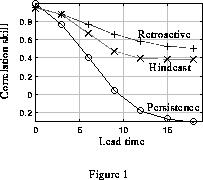
Figure 1. Correlation skills
for retroactive real time forecasts (+), hindcasts (x), and persistence
forecasts (o).
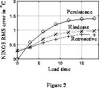
Figure 2. As in Figure 1,
except for root-mean-square error.
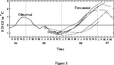
Figure 3. Forecasts of Ni¤o 3
SST based on wind stress and SST data through December 1995. The solid
line denotes the observed SST, and the 6 dashed lines the forecasts
up to lead times of 18 months initiating from July to December 1995.
[Purpose] -
[Contents] -
[Editorial Policy] -
[Next Article] -
[Previous Article]