Forecast of Pacific-Indian Ocean SSTs Using Linear Inverse Modeling

Using the methods described in Penland and Magorian (1993) and in previous issues of this Bulletin (particularly the December 1992 and June 1993 issues), the sea surface temperature (SST) anomaly in the Niño 3 region (6oN-6oS, 90o-150oW), as well as the anomaly in the Niño 4 region (6oN-6oS, 150 oW-160 oE), are predicted. A prediction at lead time t is made by applying a statistically-obtained Green function G(t) to an observed initial condition consisting of SST anomalies (SSTAs) in the IndoPacific basin. Three-month running means of the temperature anomalies are used, the seasonal cycle has been removed, and the data have been projected onto the 20 leading empirical orthogonal functions (EOFs) explaining 73% of the variance. The Niño 3 region has an RMS temperature anomaly of about 0.7oC; the inverse modeling prediction method has an RMS error of about 0.5oC at a lead time of nine months and approaches the RMS value at lead times of 18 months to two years. The COADS 1950-79 climatological annual cycle has been removed.

The predicted IndoPacific SSTA patterns based on the Dec-Jan-Feb 1995-96 initial condition for the following Mar-Apr-May, Jun-Jul-Aug, and Sep-Oct-Nov 1996, and Dec-Jan-Feb 1996-97, are shown in Fig. 1 (contour interval is 0.2oC). Figure 2a shows the predictions (light solid lines) and verifications (heavy solid lines) of the Niño 3 anomaly for initial conditions Sep-Oct-Nov and Oct-Nov-Dec 1995, and Nov-Dec-Jan and Dec-Jan-Feb 1995-96. The 1-standard deviation expected error for the prediction based on the Sep-Oct-Nov 1995 initial condition is denoted by dashed lines. Figure 2b is the same, but for the Niño 4 region. Verification and prediction do not exactly coincide at zero lead time since SSTAs are projected onto 20 EOFs for the prediction and the truncation error is included in the verification.

Consistent with the forecast published in the December 1995 issue of the Bulletin, this prediction calls for a decay of cold anomalies in the next few months. Warm anomalies are predicted to grow in the southeastern tropical Pacific and extend northward. The rapid decay of the predicted anomalies at lead times greater than six months is an indication of the uncertainty of the prediction at those lead times given current initial conditions.

Penland, C. and T. Magorian, 1993: Prediction of Niño 3 sea-surface temperatures using linear inverse- modeling. J. Climate, 6, 1067-1076.

Figures

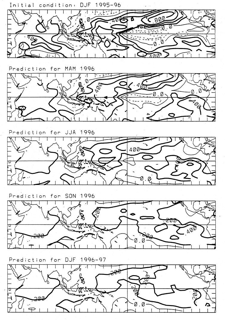
Figure 1. Linear inverse modeling forecasts of SST anomalies, relative to the standard 1950-79 COADS climatology both for the training period (1950-84) and for these forecasts. Forecast anomalies are projected onto 20 leading EOFs, based on Dec-Jan-Feb 1995-96 initial conditions (top panel). Contour interval is 0.2oC. Positive anomalies are represented by heavy solid lines, negative anomalies by dashed lines. SST anomaly data have been provided by NCEP, courtesy of R.W. Reynolds. Prediction by linear inverse modeling is described in Penland and Magorian (1993).

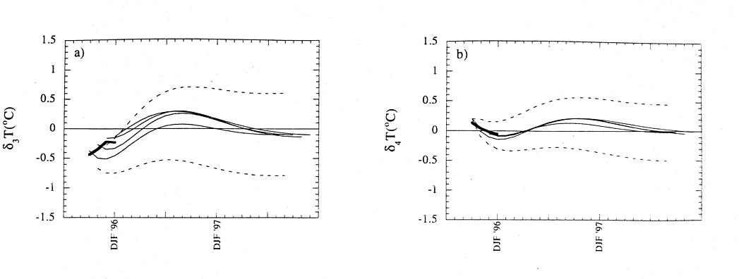
Figure 2. (a): Prediction (light solid lines) and verification (heavy solid line) of the Ni¤o 3 SSTA based on initial conditions Sep-Oct-Nov and Oct-Nov-Dec 1995, and Nov-Dec-Jan and Dec-Jan-Feb 1995-96. Dashed lines denote one standard deviation prediction error bars appropriate to a stable linear system driven by stochastic forcing for the Sep-Oct-Nov 1995 initial condition. Verification and prediction do not exactly coincide at zero lead time since SSTAs are projected onto 20 EOFs for the prediction and the truncation error is included in the verification. (b): As in (a) except for Ni¤o 4.