Complex Singular Spectrum Analysis and Multivariate Adaptive Regression Splines Applied to Forecasting the Southern Oscillation

A few years ago, Keppenne and Ghil (1992a,b; see also previous issues of this Bulletin) introduced a methodology to forecast the Southern Oscillation Index (SOI) by applying the maximum entropy method (MEM) to produce autoregressive forecasts of a set of adaptively filtered time series resulting from the application of singular spectrum analysis (SSA) to the raw monthly mean SOI. The success of this methodology has led to the development of a multivariate prediction scheme based on the same concepts, but with the substitution of multivariate SSA for univariate SSA (Keppenne and Ghil 1993, Jiang et al. 1995). The technique described herein introduces the following improvements to the linear prediction scheme used to issue the SSA/MEM predictions presented in earlier issues of this Bulletin.

First, the data base used to compute the forecasts has been extended backward from June 1945 to August 1881. Our earlier work had excluded the pre-World War II data, mainly because of numerous gaps in the Tahiti SLP. Rather than doing so here, we have developed a variation of SSA capable of handling missing values. Most data adaptive statistical prediction methods are best understood in terms of an "analog forecast" (e.g. Toth 1991, Huang et al. 1993, Livezey et al. 1994). Consequently, the extension of the data base increases the likelihood of identifying a suitable "analog" that will influence the determination of the forecast's basis functions. Figure 1 illustrates this principle by showing an adaptively filtered SOI indicator resulting from the complex SSA (CSSA) of the last 114 years (as of February 1996) of the Darwin and Tahiti SLP. The sequence of events between 1910 and 1915 presents some similarities with the early 1990s: a positive excursion of the SOI (La Nina event) is followed by two brief mild negative excursions. A strong La Nina event follows, in 1917-18. The series of circles on the righthand side of the curve shows the result of forecasting the real and imaginary parts of the SOI's leading four complex principal components (CPCs) using a variation of multivariate adaptive regression splines (MARS: Friedman 1991, Lewis and Stevens 1991, Lall et al. 1996), a nonlinear data-adaptive statistical method whose application to the SOI is discussed below. The forecast is remarkably similar to its "analog" in the 1910s and thus testifies of MARS' ability to model the dynamics of rarely occurring events. The prediction shown in Fig. 1 is markedly different from predictions obtained from either the application of linear methods to the entire data base, or from the application of MARS to the post-World War II data. Such predictions forecast near-normal conditions in the late 1990s (e.g. the Jiang et al. articles in the March and September 1995 issues of this Bulletin).

Second, in contrast with our earlier work (Keppenne and Ghil 1992a,b) in which SSA was applied to the difference between the Tahiti and Darwin normalized SLP time series, we apply CSSA to the complex time series whose real and imaginary parts consist in the Darwin and Tahiti SLP, forecast the real and imaginary parts of the resulting CPCs separately, and then take their differences to construct a forecast for the filtered SOI. This seemingly innocent procedural modification results in significant enhancements of the objective forecast skill, because taking the difference between two noisy time series increases the noise-to-signal ratio. The application of CSSA to the Darwin and Tahiti SLP followed by the subtraction of the filtered real parts of the resulting CPCs from the corresponding filtered imaginary parts circumvents this problem, thereby leading to the improved forecast skill.

Third, we have replaced the linear autoregressive MEM predictions by the nonlinear MARS methodology. MARS has advantages that significantly increase forecast skill. Among these are the ability to propagate a periodic oscillation without damping the underlying signal, and the data-adaptive capability discussed above. The latter advantage provides MARS with the capability of "analog" forecast schemes--such as radial basis functions (Casdagli 1989), nearest- neighbor bootstrap schemes (Lall and Sharma 1996) and local polynomials (Abarbanel and Lall 1996)--of reconstructing the dynamics of rarely occurring events (i.e. "recording" and "reconstructing" the character-istics of sparsely populated regions of phase space). To enhance this property, we have developed a variation of MARS in which appropriate "neighbors" of the prevailing climate conditions are identified in the phase space. The regression-splines model used to issue the predictions is then fitted to represent the mapping of each selected "neighbor" to the corresponding successor in the phase-space trajectory. More details about this specific procedure are provided in Keppenne and Lall (1995, 1996).

We use the following approach to objectively evaluate our algorithm's forecast skill. Starting with 1200 complex values in our data base, we apply CSSA with a 60-month wide time window to the data, and embed the real and imaginary parts of each CPC in 60-dimensional phase space using lagged versions of those time series as phase-space coordinates. The embedding phase spaces are then searched for the nearest two hundred neighbors of the time series' last points and MARS models are fitted using the phase-space coordinates of the neighbors as predictor variables and their temporal successors as predictands. A 60-month forecast is then issued for each real and imaginary part. The corresponding forecast for the SOI is obtained by convoluting the extended (as a result of the forecast's issuance) CPCs with the corresponding CEOFs, and subtracting the real part of the resulting time series from its imaginary part. The scheme is then repeated with one more complex number in the data base representing the following monthly mean SLP values at Darwin and Tahiti, and a new 60-month forecast is issued. This procedure is repeated until the data base is exhausted and the resulting 168 sets of eight forecasts (one for each real and imaginary part of the leading four CPCs) are used to objectively measure the procedure's predictive ability. Note that this is a "retroactive real-time" simulation, in that future "analogs" are not used.

Figure 2 illustrates the differences in skills between various forms of MARS models. In it, the average error of applying a 60-month forecast with either one of the following methods is compared to the average error of a persistence forecast: (a) MEM as in Keppenne and Ghil (1992a,b), (b) MARS with interaction level one, (c) MARS with interaction level two, and (d) MARS with interaction level three. MARS employs multivariate cubic spline basis functions for regression. The interaction level determines the types of terms that are considered in forming a tensor product across variables or coordinates. Inclusion of higher- order interaction terms indicates the presence of an increasing amount of nonlinearity in the underlying dynamics.

The forecasts in Fig. 2 are for the time series reconstructions involving the leading four CPCs rather than for the monthly mean SOI itself or for its five- month running mean. Note that all three types of MARS models dramatically outperform the MEM models at short (<30-month) leads. All forms of MARS models have comparable skills for most lead times, although the higher-interaction-level models slightly outperform the lower-interaction-level ones.

Figure 3 shows eight 60-month lead SOI forecasts issued at intervals of 24 months between August 1981 and August 1993, including the relatively recent (but not most current) forecast based on data up to November 1995. The solid line in Fig. 3 denotes the last 15 years of the five-month running-mean SOI. Each series of connected circles is a 60-month lead forecast. Note how well the 82-83 and 86-87 El Nino events could have been forecasted at leads of several years. The forecast skill corresponding to the prediction of the 1985 and 1988 La Nina events is also impressive. However, the skill is much lower in the early 1990s, where all our forecasts miss the doubly recurring mild El Nino event. This fact is not surprising, since the interannual variability from the mid 1960s to the late 1980s has been highly regular (Fig. 1). Indeed, one has to go back almost 80 years in the data base to encounter an event reminiscent of the recent conditions (Fig. 1). As discussed above, the strong La Nina event predicted for the late 1990s (Fig. 1) is a result of our variation of MARS' ability to produce "analog" type forecasts, a capability not present in the SSA-MEM approach of Keppenne and Ghil (1992a,b).

Compared with the forecast issued 3 months ago in the December 1995 issue of this Bulletin, the present forecast is reasonably similar. The strength of the La Nina is now predicted to be slightly less than before (but still substantial), and to peak somewhat earlier--in early to middle 1997.

Abarbanel, H.D. and U. Lall, 1996: Nonlinear dynamics of the Great Salt Lake: system identification and prediction. Clim. Dyn., in press.

Casdagli, M., 1989: Nonlinear prediction of chaotic time series. Physica D, 35, 335-356.

Friedman, J.H., 1991: Multivariate adaptive regression splines. Ann Stat, 19, 1-50.

Huang, J.P., Y.H. Yi, S.W. Wang and J.F. Chou, 1993: An analog-dynamic long-range numerical weather prediction system incorporating historical evolution. Q J R Met. Soc., 119, 547-565.

Jiang, N., M. Ghil and D. Neelin, 1995: Forecasts of equatorial Pacific SST using an autoregressive process using singular spectrum analysis. Exp. Long-Lead Forcst. Bull., 4, No. 1, 24-27.

Keppenne, C.L. and M. Ghil, 1992a: Forecasting extreme weather events. Nature, 358, 547.

Keppenne, C.L. and M. Ghil, 1992b: Adaptive Spectral Analysis and Prediction of the Southern Oscillation Index. J. Geophys. Res., 97, 20449-20554.

Keppenne, C.L. and M. Ghil, 1993: Adaptive filtering and prediction of noisy multi-variate signals: an application to atmospheric angular momentum. Intl. J. Bifurcations and Chaos, 3, 625-634.

Keppenne, C.L. and U. Lall, 1995: A new methodology to forecast paleoclimate time series with application to the Southern Oscillation index. EOS Trans AGU. 1995 Fall Meeting Supplement, 76, F327.

Keppenne, C.L. and U. Lall, 1996: Complex singular spectrum analysis and multivariate adaptive regression splines applied to forecasting the Southern Oscillation. J. Clim., 9, submitted.

Lall, U. and A. Sharma, 1996: A nearest-neighbor bootstrap for resampling hydrologic time series. Water Resources Res., in press.

Lall, U., T. Sangoyomi and H.D. Abarbanel, 1996: Nonlinear dynamics of the Great Salt Lake: nonparametric short term forecasting. Water Resources Res., in press.

Lewis, P.A.W. and J.G. Stevens, 1991: Nonlinear modeling of time series using multivariate adaptive regression splines (MARS). J. Amer. Stat. Assoc., 86, 864-877.

Livezey, R.E., A.G. Barnston, G.V. Gruza and E.Y. Rankova, 1994: Comparative skill of 2 analog seasonal temperature prediction systems: Objective selection of predictors. J. Clim., 7, 608-615.

Toth, Z., 1991: Estimation of atmospheric predictability by circulation analogs. Mon. Wea. Rev., 119, 65-72.

Figures

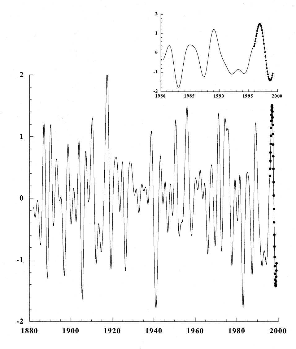
Figure 1. Adaptively filtered Southern Oscillation Index (SOI) time series resulting from the complex singular spectrum analysis (CSSA) of the monthly mean Darwin and Tahiti sea-level pressure (SLP) data through February 1996 (solid). Note the similarity between the two brief negative excursions of the filtered SOI following the strong La Nina event in the early 1910s and the recent conditions. The application of a variant of multivariate adaptive regression splines (MARS) to the real and imaginary parts of the leading four complex principal components (CPCs) resulting from the CSSA yields a forecast (circles on right side of curve) reminiscent of the conditions that dominated in the late 1910s (a strong La Nina) and illustrates MARS' capability to model the conditions of rare events.

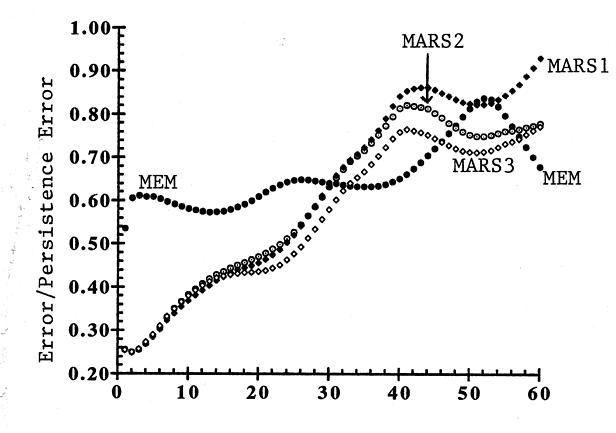
Figure 2. Ratio of the average forecast error of 60-month forecasts issued with either MEM (full circles), interaction-level-one MARS models (full diamonds), interaction-level-two MARS models (open circles) and interaction-level-three MARS models (open diamonds), to the average error of a same-lead persistence forecast. Shown is the forecast error for the adaptively filtered time series obtained by convoluting each of the leading four CPCs with the corresponding complex empirical orthogonal function (CEOF). For example, the average error of interaction-level-three MARS forecasts grows from about 0.25 times that of a persistence forecast at one-month lead to about 0.8 times it at 60-month lead.

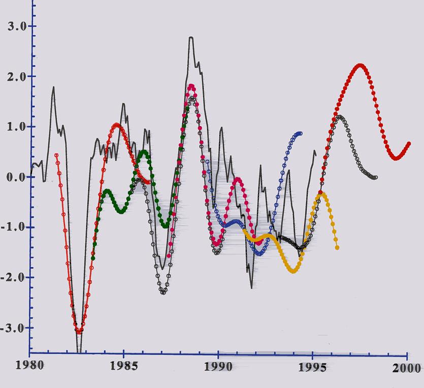
Figure 3. Five-month running-mean SOI (solid) and series of eight 60-month lead forecasts (series of connected circles) obtained by combining the forecasts resulting from the application of cubic MARS models to the real and imaginary parts of the leading four CPCs resulting from the Darwin and Tahiti data's CSSA. See text.