[Previous Article]
[Next Article]
Forecasts of Tropical Pacific SST Anomalies
Using a Statistical (EOF) Iteration Model
contributed by B. Zhang1 and Jianfu
Pan2
1Institute of Atmospheric Physics, Chinese Academy of Sciences, Beijing, China
2Climate Prediction Center, NOAA,
Camp Springs, Maryland
A statistical model is used to produce a time series of
SST anomaly (SSTA) forecasts, based on a temporal EOF iteration scheme
(Zhang et al. 1993). The method is a predictive form of singular spectrum
analysis (SSA; Vautard and Ghil 1989), and has conceptual similarity to
an analogue method. In this method, EOFs are computed using a correlation
matrix derived from a specially constructed data matrix. This matrix contains
data from a single spatial point that increase temporally both with row
and column index (as in SSA). In the last column of the last row, a first
guess of a future (unknown) value of the time series is given--perhaps
the climatological mean. When EOFs are computed and the raw data are reconstructed
using a truncated set of modes, the unknown value is determined in keeping
with the patterns of the EOFs. This process is reiterated using the latest
guess of the unknown value until the changes in that value with subsequent
iterations become smaller than a prescribed amount. Then the same procedure
is carried out for the next future time point, accepting the previously
forecast time point as if it were observed. In essence, the method uses
past temporal patterns of the variable to forecast future values.
Each of the first 6 principal components (PCS) of the
tropical Pacific basin SST are forecast; these are then used to reconstruct
the SSTA pattern forecasts. Using SST data spanning from 1970 (obtained
from the Climate Prediction Center), 174 forecasts with various beginning
and ending times have been made at lead times ranging from 1 to 24 months,
respectively. For example, 1 month lead forecasts begin in January 1982
and end in June 1996, 2 month lead forecasts begin in February 1982 and
end in July 1996, and so on.
The forecast skill of the model has been evaluated, as
shown in Fig. 15-1 of the December 1994 issue of this Bulletin. It was
demonstrated that the tropical Pacific SSTA can be forecast fairly well
up to 9 months lead, especially in the eastern portion of the basin.
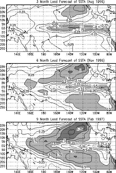
Figure 1 shows 3, 6 and 9 month lead tropical Pacific
SSTA forecasts for August and November of 1996, and February 1997. The
forecasts show below normal SSTs over the eastern part of the equatorial
Pacific. A magnitude of -1EC is indicated in 3 month lead forecasts. These
magnitudes decrease after August 1996, and a horseshoe-shaped pattern of
positive SSTA in the northern and southern hemisphere subtropical Pacific
and western equatorial Pacific surrounds the negative eastern equatorial
SSTA.
The area average Nino 3 and Nino 4 SSTAs for all 174 forecasts
at 3-, 6- and 9-month lead are shown in Figs. 2 and 3, respectively, along
with corresponding observations (solid lines). The forecasts are for negative
SSTs in the next 3 months (through August) in Nino 3, and near normal SSTs
in Nino 4. Subsequent changes are in the positive direction. This implies
that the Nino 3 region will become closer to normal and the Nino 4 region
slightly above normal for boreal winter 1996-97.
References
Vautard, R. and M. Ghil, 1989: Singular spectrum analysis
in nonlinear dynamics, with applications to paleoclimatic time series.
Physica D Amsterdam, 35, 395Ł424.
Zhang, B., J. Lie and Z. Sun, 1993: A new multidimensional
time series forecasting method based on the EOF iteration scheme. Advances
in Atmospheric Sciences, 10, 243-247.
Fig. 1. Three, 6 and 9 month lead SSTA forecasts
for August (top) and November (middle) of 1996, and February 1997 (bottom).
Contour interval is 0.25EC. Light shading denotes anomalies of 0.5EC to
1.0EC in amplitude, dark shading 1.0EC and higher.
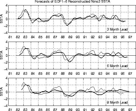
Fig. 2. Predicted and observed SSTA time series
for Nino 3 for lead times of 3 (top), 6 (middle) and 9 (bottom) months,
based on reconstructions of the first 6 EOF modes. Observed time series
are indicated by the solid line, and forecasts by dots.
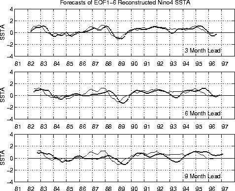
Fig. 3. As in Fig. 2, except for Nino 4.